The Repeater Mystery
One of the central problems of networking is distance: the farther a message has to travel, the more it degrades and the more likely it is to be lost. In ordinary networks, one way of dealing with this is the repeater: a device that receives a weakened signal, boosts it, and sends it on. But in practice “boosting” is really just another word for refreshing the signal by copying its information - taking, say, an incoming light particle and making more copies of it. It is a bit like restoring a painting: you inspect the fading pigment, work out what was there, and apply fresh paint. Classical communication survives by refreshing information.
Quantum communication cannot work that way. An unknown quantum thing cannot be perfectly cloned. This is the no-cloning theorem of quantum mechanics. Many readers may already feel the shape of this idea from the famous uncertainty principle: a particle’s position and momentum cannot both be known exactly at the same time. If one could clone an arbitrary quantum object, one could measure position on one copy and momentum on the other, apparently dodging the restriction. [1] So the central engineering question becomes: how do you build a network once copying is no longer allowed?
What, then, is a quantum repeater in a world where copying is forbidden, and more broadly, what is quantum networking? This essay will answer these questions in a simplified but serious way. We will avoid formalism, but not the real structure of quantum information theory. The mathematics will stay light. The ideas will not. Quantum mechanics is famous for its weirdness as we already saw in the “Is Reality Real - Experimentally Speaking?” essay, but that weirdness is not just something to puzzle over: it can be turned into engineering.
Quantum Mechanics in a Pea-Shell
To understand quantum networking, we first need the bare minimum of quantum mechanics.
One magic coin
Fig. 1. A table of a magic coin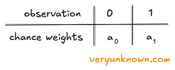
The table has two columns for the only outcomes we can ever observe: 0 or 1. Beneath them sit the chance weights. To get the probability of an outcome, we square its weight [2]. Why not write probabilities directly? Because we are quietly introducing the basic rules of quantum mechanics. In full physics, this would not be a magic coin but perhaps a particle, and the columns might mean “the particle is here” and “the particle is there.” But the same kind of table would still appear. So the magic coin is not just a metaphor. It is quantum mechanics with the physical details abstracted away. A classical coin is either heads or tails, whether we know it or not. A quantum coin — a qubit — is described by the whole table at once. If all the weight sits in 0, measurement gives 0 with certainty. If all the weight sits in 1, it gives 1 with certainty. The interesting case is when both columns carry weight. Then the table is the full description.
Two magic coins
Fig. 2. A table of two qubits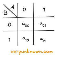
Each box gives the chance weight for a joint outcome: 00, 01, 10, or 11. Observation is easy to describe in this picture. If we observe coin A and get 0, we keep only the A=0 column and throw away the other one. If we observe A and get 1, we keep only the A=1 column. Likewise, observing B means keeping one row and discarding the other. After that, we rescale the surviving weights so the total probability adds up to 1. In this table language, measurement means - delete everything inconsistent with what you saw.
Fig. 3. A table of two qubits in 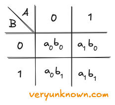
‘product state’
Here is the key fact: in this multiplication case, observing one coin does not change the odds of the other. If we observe A and keep only one column, both surviving entries in that column carry the same extra factor, either a0 or a1. When we rescale, that common factor cancels out. So coin B keeps the same odds it had before. Learning A tells us nothing about B. If a two qubit table can be rewritten in the above multiplicative form, we can think of coins A and B being independent and just sitting side by side. That is what independence looks like in this language.
Fig. 4. A table of two qubits in 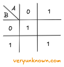
’entangled state'
Actions on a magic coin
Fig. 5. Actions on a qubit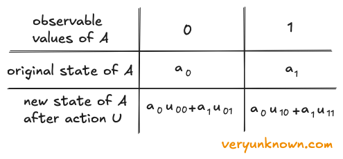
The important point is simple: an allowed quantum action remixes the old chance weights into new ones by multiplying and summing. It acts on the whole table at once. The same picture carries over to two coins. Now there are four boxes instead of two, so the action remixes four old chance weights into four new ones [4].
This may look suspiciously simple, but it is not a fake rule invented for convenience. It is the basic shape of actions that can happen in quantum mechanics. In real physics one would usually write something more like \(u_{ij}(t)\), because the action is some physical process which evolves over time, and the entries \(u_{ij}\) might come from quite complicated physical machinery. We are hiding all of that on purpose. For our purposes, the entire mess of actual physics can sit behind a table of numbers called \(u_{ij}\).
In this essay we will not worry about what physical device realizes the qubit, or what electromagnetic field or Hamiltonian sits underneath the hood. We will just keep the essential rules: a qubit is a table of chance weights, and probabilities come from squaring them, two qubits form a joined table with four entries, observation deletes incompatible entries, allowed actions remix the weights by multiplying and summing. This is the core of quantum mechanics and already enough structure to start doing useful and interesting things.
Quantum Circuits
The tables above are enough to play the game. But once several actions happen in a row, the bookkeeping starts to get in the way. ‘‘Quantum circuits’’ are the same actions, just drawn as pictures. No new physics or math is being added. We are just switching to a more visual, easier-to-follow way of keeping track of what is happening.
See below a few circuits in Fig. 6, Fig. 7., and Fig. 8. A circuit is read from left to right. Each horizontal line is one magic coin. A box placed on a line means ‘‘apply this one-qubit action here.’’ If two lines are linked, the action involves both qubits. Under the hood, the same table-remixing rules are still doing the work, and one can define the \(u_{ij}\) values for each of them. The boxes are called ‘‘gates’’.
Three basic gates
Let’s have a look at a few gates which we will need
Fig. 6. X Gate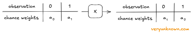
Fig. 7. H Gate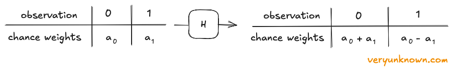
Fig. 8. CNOT Gate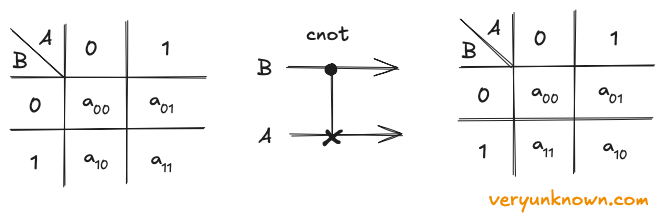
There are other useful gates out there, but these will be enough for our purposes.
Making entanglement
We now have all the tools we need, so let us see what we can build with them. To start with, we have already talked about entangled states, but how do we actually make one? Here is a simple recipe.
Fig. 8. Entanglement circuit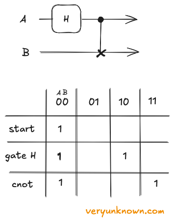
At the start, only 00 is alive. After the H step, the state has split into two branches. After the CNOT, those branches line up as 00 and 11. We have arrived at a system which starts with definite state, and outputs an entangled one!
Quantum Teleportation
This brings us to the core of the story: how to do networking without cloning. The trick is teleportation. Teleportation sounds dramatic, but the idea is pretty practical. We are not sending matter through thin air. We are moving the state of one qubit, \(\psi\), onto another qubit far away.
Fig. 9. Teleportation circuit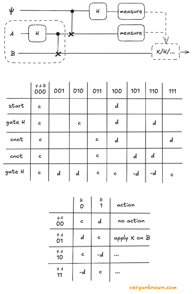
Only once the shared pair is in place do we bring in \(\psi\), with unknown chance weights c and d. The sender lets \(\psi\) interact with A, and then measures both of them. After that, the sender is done with the quantum part of the protocol. The original state is no longer sitting on the sender’s side as after measurement \(\psi\)A is in a definite state. What remains there are just two ordinary measurement bits, which can be sent across a classical channel.
The big table in Fig. 9. is the full bookkeeping for the three-qubit system. Each row is one moment in the circuit. Its job is to show how the unknown weights c and d get shuffled around without ever being read out directly. You do not need to chase every entry. The key point is the last row: after the sender’s steps, qubit B already holds the right state, but with a small known twist. That is what the little ‘‘apply action’’ table is for. Read the two measured bits \(\psi \)A, find the matching row, and apply the listed fix on B. The correction is always something simple: maybe do nothing, maybe apply an X flip, etc. The receiver is not rebuilding the state from scratch. The receiver is only undoing a known twist. After that correction, B is in exactly the state that \(\psi\) started in. That is the teleportation!
Why call this ‘’teleportation’’ at all? Because the only ordinary data sent after the measurement are two classical bits, and two bits are nowhere near enough to describe a general qubit state. A general qubit is not one of four fixed options; it can sit in a continuous range of possible states. So those two bits are not a full description of the state. They are only the instructions for which final correction to apply to the far qubit. And there is no hidden copying trick here. At no point do we have two perfect copies of the unknown state. The sender has to measure \(\psi\) and A, which consumes the original. The state moves from one place to another, but it is never duplicated.
This idea is also surprisingly recent. Quantum mechanics is a 1920s theory, but the standard teleportation protocol was proposed only in 1993. It already feels more like network engineering than physics: first create entanglement across a noisy link, retry if the traveling qubit is lost, and only then use that shared resource, together with two classical bits, to move a fragile quantum state without ever cloning it.
Quantum Repeater
This brings us back to the original mystery: in a no-cloning world, what could a repeater even be? In an ordinary network, a repeater can boost a signal or copy bits onward. A quantum repeater cannot. Teleportation helps, but it still requires an entangled pair shared across the link, so some qubit has to travel a real physical distance. Over long distances, that gets hard: photons are lost, noise builds up, and eventually the link is just too long. So a quantum repeater avoids one giant link. Instead, it builds shorter entangled links and stitches them together in the middle.
Here is the basic recipe. We will not stop here to draw the full circuit or run the full table derivation, even though by this point we already have everything we would need to do exactly that. Instead, we will stay at the higher level and look at the main idea. At location A, create an entangled pair \(A_0\) and \(A_1\). Keep \(A_0\) and send \(A_1\) to a middle station C. Independently, location B creates another entangled pair \(B_0\) and \(B_1\). It keeps \(B_0\) and sends \(B_1\) to the same middle station C. If one of those traveling qubits is lost on the way, we simply remake entangled pair and resend the qubit. That is much easier than asking one qubit to survive the whole trip from A to B.
Now comes the key move. At C, we perform on \(A_1\) and \(B_1\) the same kind of joint mix-and-measure trick that powers teleportation. This consumes the two middle qubits, but it pushes the entanglement outward. In the technical language, C performs entanglement swapping. After that, \(A_0\) and \(B_0\) form an entangled pair, even though they never met and neither one travelled the full distance. That is the whole point: the long entangled link from A to B has been built out of two shorter links, one from A to C and one from C to B. In this simple setup, the reachable distance has doubled.
So a quantum repeater does not beat loss by copying qubits. It beats loss by creating entanglement in short hops, then tying those hops into a longer one. It is not a machine for boosting a quantum signal. It is a machine for moving entanglement outwards until two faraway endpoints are entangled.
Where the Magic Becomes Technology
If you have made it this far, you have already come a surprisingly long way. Starting from a toy ‘‘magic coin’’, we built up the logic of qubits, saw why entanglement is unusual, and followed that thread through circuits, teleportation, and finally quantum repeaters. Along the way, we did not just learn a few isolated quantum tricks. We started to build a real toolkit. The same small set of quantum rules, the same basic circuit moves, already let us assemble surprising and powerful things. That is enough to see the larger point: quantum mechanics may first look like pure strangeness, but this strangeness can be harnessed for engineering. Quantum magic can be turned into technological magic. Here we focused on networking - on how to move, share, and extend fragile quantum states across distance without ever cloning them. But this is only one thing those same rules can do. Just as ordinary computing is not only about sending bits but also about computing with them, the quantum world has another great story waiting beyond the network: computation on qubits themselves. That, however, is a story for another day.
[1] The no-cloning theorem is actually even more fundamental than this intuition suggests. It does not depend on the uncertainty principle, but follows directly from the basic rules of quantum mechanics. We will return to this briefly later; see footnote [4].
[2] More precisely, the weights are complex numbers, and the probability of an outcome is the squared magnitude of its weight. But for the purposes of this essay, that extra complexity does not matter.
[3] Strictly speaking, this table should be multiplied by one overall constant so that the squared chance weights add up to 1, in this case that constant would be \(1/\sqrt{2}\). In this essay we will suppress such overall constant for legibility.
[4] The no-cloning can already be seen from the existing basic rules. Very briefly, in the table language, cloning would mean taking one arbitrary qubit together with a qubit in definite state, and then applying one fixed remixing rule that produces two independent copies as in table in Fig. 3. It’s quite easy to find that there is no such remixing rule possible, but we will skip the details for brevity.