What’s at stake
We will talk about an experiment of the sort for which the 2022 Nobel Prize in physics was awarded. It’s an experiment that contradicts two very cherished “common sense” assumptions about how nature is, forcing us to give up at least one of them.
The first one is that things have a clearly defined existence, even when we are not looking. Like the question - “if a tree falls in a forest, does it make a sound if no one is looking?” The answer should be obvious - yes. To rephrase even more vividly - “if no one is looking, is the tree standing, or has it fallen on the ground?” Again clearly - it should be one or the other. Or if we put a cat in a dangerous box and closed it - is the cat dead or alive within it before anyone looks? Common sense deriving from experience tells us that it is indeed exclusively one of the two. We are in good company - Einstein thought so too.
The second one is the idea of “locality” - only adjacent things interact. This might feel a bit less intuitive because we experience in our daily lives such mundane examples as wireless communication. Two things interact seemingly instantaneously at a distance. However, this perception is not accurate. For example, when a space probe from Mars sends back images to Earth it takes about 10 minutes to reach earth. It takes time for the signals to travel - interaction between the space probe’s antenna and the antenna on Earth is not instantaneous. The radio wave (aka “electromagnetic” wave) is traveling with some finite speed from an adjacent point to the next adjacent point. The reason why on Earth such communication looks instantaneous is that the travel speed is very fast compared to distances on Earth - e.g. an electromagnetic wave could travel about 7 times around Earth in a second. The assumption of “locality” is a cornerstone of modern physics - in particular General Relativity and Quantum Field Theory. These theories are fantastically successful at describing and predicting experimental outcomes. In other words - “locality” as an assumption is extremely successful at explaining experimental observations. We are in good company on this point too - Newton also thought this reasonable.
Both assumptions taken together are known as “local realism”. “Realism” is just “common sense”, while “locality” is also pretty common sense, but also a spectacularly successful assumption of modern physics. So far so pretty boring. So what is Nobel Prize worthy here?
Here is the kicker - experimental facts contradict “local realism”. Ie. “local realism” is experimentally refuted. This leaves us in a strange place. We need to give up at least one of them, but which one do we give up? Modern theories like Quantum Field Theory does not assume “realism”, but it does assume “locality”, and is experimentally extremely successful. So should we give up “realism”? But that is crazy - giving up the notion that “things are not this or that”. But if we want to keep to realism, we need to give up our most successful physical theories. A wacky place to be in, but such are things.
And this is what we will be looking into - the experimental setup and associated logic leading to the conclusion that “local realism” is false.
The Experiment
The experiment is as follows [1] - we have a type of measurement device that can be set to one of two settings - “1” and “2”. It will measure a particle and flash orange or blue color light as a measurement outcome. There are three labs, each with a measuring device. In addition, there is one emitter of particles - when someone presses a button on the emitter it emits three particles, and each one of them travels to the corresponding lab, so each lab gets one particle for a measurement. In each lab scientist does a measurement with the lab’s device on said particle - first, the scientist randomly selects one of the two settings and then does the measurement. They each write down their setting and the outcome of the measurement. The three labs will be located far apart - to make sure that when scientists do measurements, they do not affect the measurements of the other labs [2]. This experiment is repeated many times. At the end, scientists travel, meet, and create a table of data on what settings they had set and what they measured for each individual experiment. What will they see?
A bit on notation. We will write things like “112” to mean “lab one had setting 1, lab two had setting 1, lab three had setting 2” when doing the measurements for a single experiment. We will summarise the result of three measurements as “🟠🔵🟠”, which will mean “lab 1 saw orange measurement, lab 2 saw blue measurement, lab 3 saw orange measurement”.
Here are the following experimental results:
- if settings were set to 122, 212, or 221, then scientists measured - 🟠🟠🟠 or 🔵🟠🔵 or 🟠🔵🔵 or 🔵🔵🟠
- if settings were set to 111 then scientists measured - 🔵🔵🔵 or 🟠🔵🟠 or 🔵🟠🟠 or 🟠🟠🔵
These are the results of experiments [3]. Now let us apply some reasoning to see what will happen if we assume “realism”. Each particle will have some property “X” which will cause the measurement device to blink orange or blue. Our argument is not affected by what the specific physical property is - it will suffice for us to describe what measurement outcome this property “X” will cause on a device. We will write “🔵🟠” to indicate that “if the device setting is 1 the particle will cause the device to blink blue, but if the device setting is 2 the particle will cause the device to blink orange”. There are only four possible combinations - 🟠🟠 or 🔵🟠 or 🟠🔵 or 🔵🔵. Now, there are 3 such particles, so we will write 🟠🟠/🟠🔵/🔵🟠 to mean - “first particle will cause orange measurement if a device is set to 1 or 2, the second particle will cause orange measurement if the setting is 1, blue if the setting is 2, the third particle will cause blue measurement if the setting is 1, orange if the setting is 2”.
Let us build a table of all possible combinations of what the 3 particles could be during each individual experiment. See column “Particles”. In the table, the next four columns show what would be the outcome of an experiment for given settings 112, 212, 221, and 111 given the particle properties. The final four columns show the following - does the given row of how particles are fit experimental observations as outlined above.
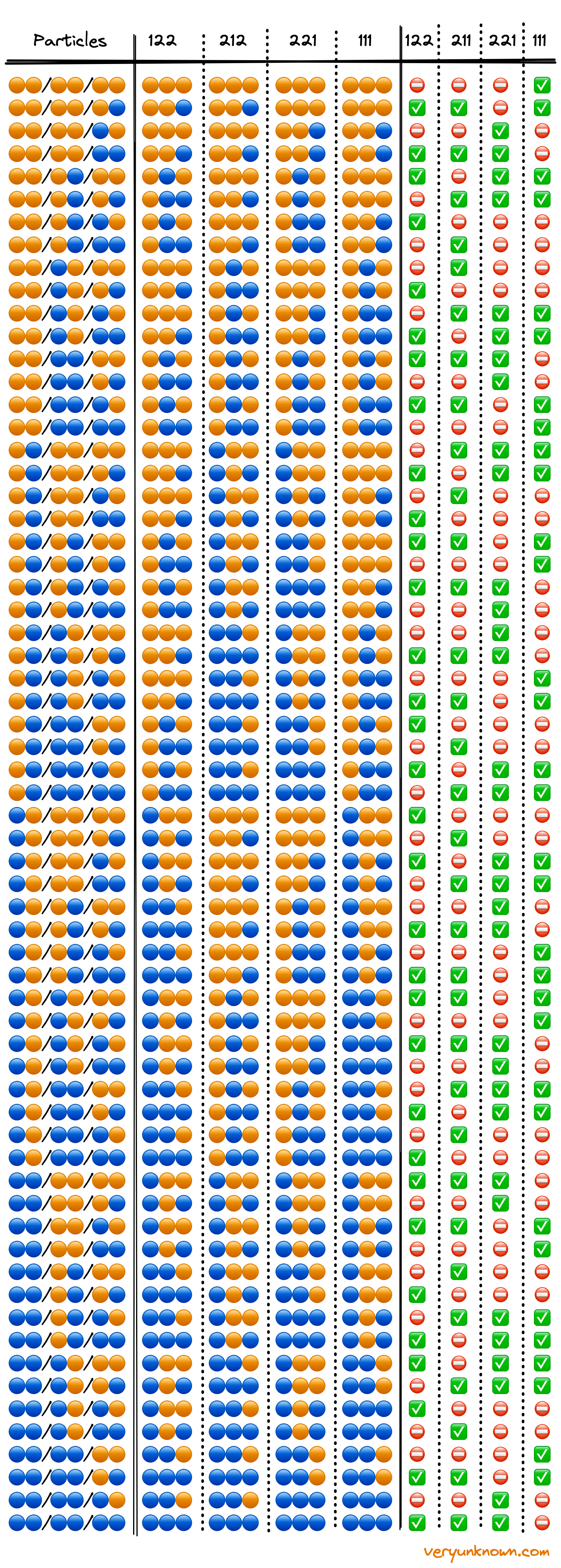
Table 1. Possible particle setups and if experimental outcomes match expected results given “local realism” assumption
When looking through the table, the following observation of the last four columns is the key - all rows have at least one case which does not match experimental observation. As the settings are selected at random it would mean that at least 1 in 4 measurements on average would contradict actual observations. This contradiction came from following some reasoning from the assumption of “local realism” being true. Thus “local realism” must be false.
Where next?
Have such type experiments actually been executed? The answer is yes - thus the Nobel Prizes. So “local realism” is false - but where do we go next from this? Give up “locality”? But that would imply giving up a cornerstone of modern physics theories - which have been stunningly successful. Give up “realism”? That just contradicts common sense. There is no straightforward answer - beyond being amazed that the world is more surprising than we could have ever imagined.
Appendix: For the quantum mechanics buffs
What does quantum mechanics have to say about this experiment? Eg. the property “X” could be electron spin. In the braket notation, we will use “bar” over the letter to indicate the “opposite”. E.g. \(\ket{\uparrow}\equiv\ket{z}\), and \(\ket{\downarrow}\equiv\ket{\bar{z}}\). We will cheerfully ignore normalization factors for state vectors to minimize clutter. To recap for spin:
$$ \ket{x} = \ket{z}+\ket{\bar{z}}, \ket{\bar{x}} = \ket{z}-\ket{\bar{z}} $$ $$ \ket{y} = \ket{z}+i\ket{\bar{z}}, \ket{\bar{y}} = \ket{z}-i\ket{\bar{z}} $$ With a bit of rearrangement $$ \ket{z} = \ket{x}+\ket{\bar{x}}, \ket{\bar{z}} = \ket{x}-\ket{\bar{x}} $$ $$ \ket{z} = \ket{y}+\ket{\bar{y}}, \ket{\bar{z}} = i(\ket{y}-\ket{\bar{y}}) $$
The state of the particles is [4] $$ \ket{particles} = \ket{z}\ket{z}\ket{z} - \ket{\bar{z}}\ket{\bar{z}}\ket{\bar{z}} $$
When the device is measuring “Setting 1” it’s measuring in x direction, while “Setting 2” is y direction. If the device measures a state with a “bar” it flashes blue, otherwise orange. Let us say devices are set to measure 122 settings. Changing the basis and with a bit of tedious but straightforward algebra
$$ \ket{particles} = \ket{z}\ket{z}\ket{z} - \ket{\bar{z}}\ket{\bar{z}}\ket{\bar{z}} = $$ $$ = (\ket{x}+\ket{\bar{x}})(\ket{y}+\ket{\bar{y}})(\ket{y}+\ket{\bar{y}}) - (\ket{x}-\ket{\bar{x}})i(\ket{y}-\ket{\bar{y}})i(\ket{y}-\ket{\bar{y}}) = $$ $$ =\ket{x}\ket{y}\ket{y}+\ket{\bar{x}}\ket{\bar{y}}\ket{y}+\ket{\bar{x}}\ket{y}\ket{\bar{y}}+\ket{x}\ket{\bar{y}}\ket{\bar{y}} = $$ $$ =\ket{🟠}\ket{🟠}\ket{🟠}+\ket{🔵}\ket{🔵}\ket{🟠}+\ket{🔵}\ket{🟠}\ket{🔵}+\ket{🟠}\ket{🔵}\ket{🔵} $$
This matches experimental observations. Similar algebra follows for 212 and 221 settings. But what about 111 case. Let us follow the algebra.
$$ \ket{particles} = \ket{z}\ket{z}\ket{z} - \ket{\bar{z}}\ket{\bar{z}}\ket{\bar{z}} = $$ $$ = (\ket{x}+\ket{\bar{x}})(\ket{x}+\ket{\bar{x}})(\ket{x}+\ket{\bar{x}}) - (\ket{x}-\ket{\bar{x}})(\ket{x}-\ket{\bar{x}})(\ket{x}-\ket{\bar{x}}) = $$ $$ =\ket{\bar{x}}\ket{x}\ket{x}+\ket{x}\ket{\bar{x}}\ket{x}+\ket{x}\ket{x}\ket{\bar{x}}+\ket{\bar{x}}\ket{\bar{x}}\ket{\bar{x}} = $$ $$ =\ket{🔵}\ket{🟠}\ket{🟠}+\ket{🟠}\ket{🔵}\ket{🟠}+\ket{🟠}\ket{🟠}\ket{🔵}+\ket{🔵}\ket{🔵}\ket{🔵} $$
Which also matches experimental observations in vivid contrast to Table 1.! Quantum entanglement for the win!
[1] N. Mermin, 1990
[2] Labs are far enough so that measurement cannot affect particles at other labs as there is not enough time for some interaction to travel to other labs before said remote particles get measured themselves. See more on the maximum speed of propagation in “Inventing special relativity”.
[3] Setting cases 112, 121, 211, 222 does not affect the argument, so we ignore them
[4] As investigated by D. Greenberger, M. Horne, and A. Zeilinger, 1989.