Computing
Computing is pervasive nowadays, and exhibits surprising versatility. It can do large scale weather simulations predicting storms and saving lives. It can generate beautiful animated movies. It can provide an opponent for playing chess or poker. We could keep going and going describing what a computing machine could do. This raises a question - if computing can express so much, what is core of computing? Antoine de Saint-Exupéry, the author of “Little Prince”, said that “Perfection is achieved, not when there is nothing more to add, but when there is nothing left to take away.” This is the journey which we will embark upon. We will take away everything until only the perfect heart of computing is left.
Cutting and pasting is everything
What can be more natural place to start exploring of what can be expressed than by looking at juggernaut of expressing - a language. In language we have words, and we have grammar. Words give meaning, while grammar tells how to stitch words together. When all is tied together, we get a sentence. We will stitch things together by cutting and pasting. Lets look at a simple example in Fig 1.
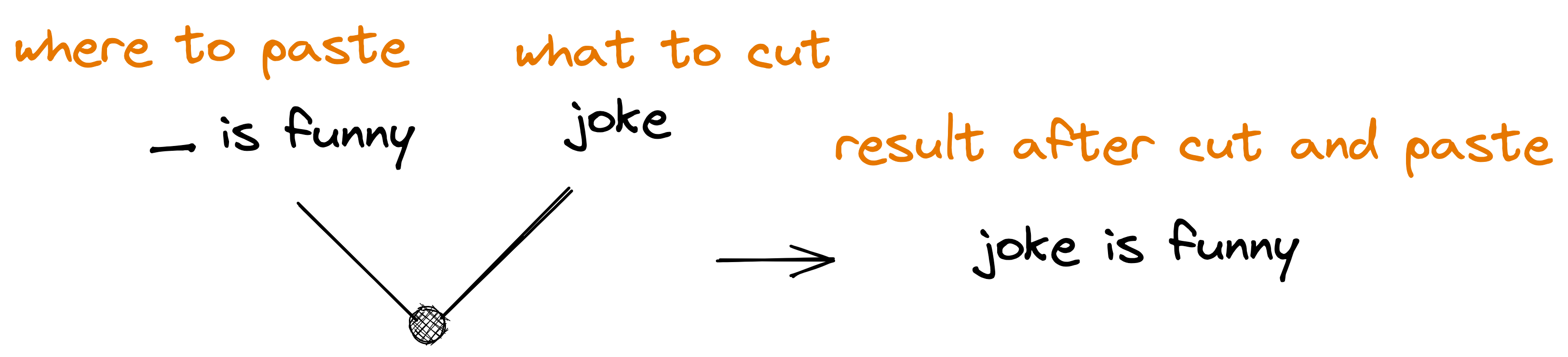
Fig 1. Simple cut-and-paste pattern
For cutting and pasting we need two things. First, we need somewhere to paste to. In Fig 1. it’s the pattern on the left of black circle. We will call the pattern on the left a “function”. Second, we need the thing we will be cutting for pasting. In Fig 1. it’s the pattern on the right of black circle. We will call pattern on the right “data”. The black dot and the “v” indicate that we are doing “cut and paste” - “cut the thing on the right, and paste it in pattern on the left and write down the final result”. Notice how in Fig 1. the pattern was on the left. It is important! We cut the thing on right and paste it in the pattern on the left. Never the other way around! What if we have a pattern with more than one slot? Lets see Fig 2.
Fig 2. Pattern with more than one slot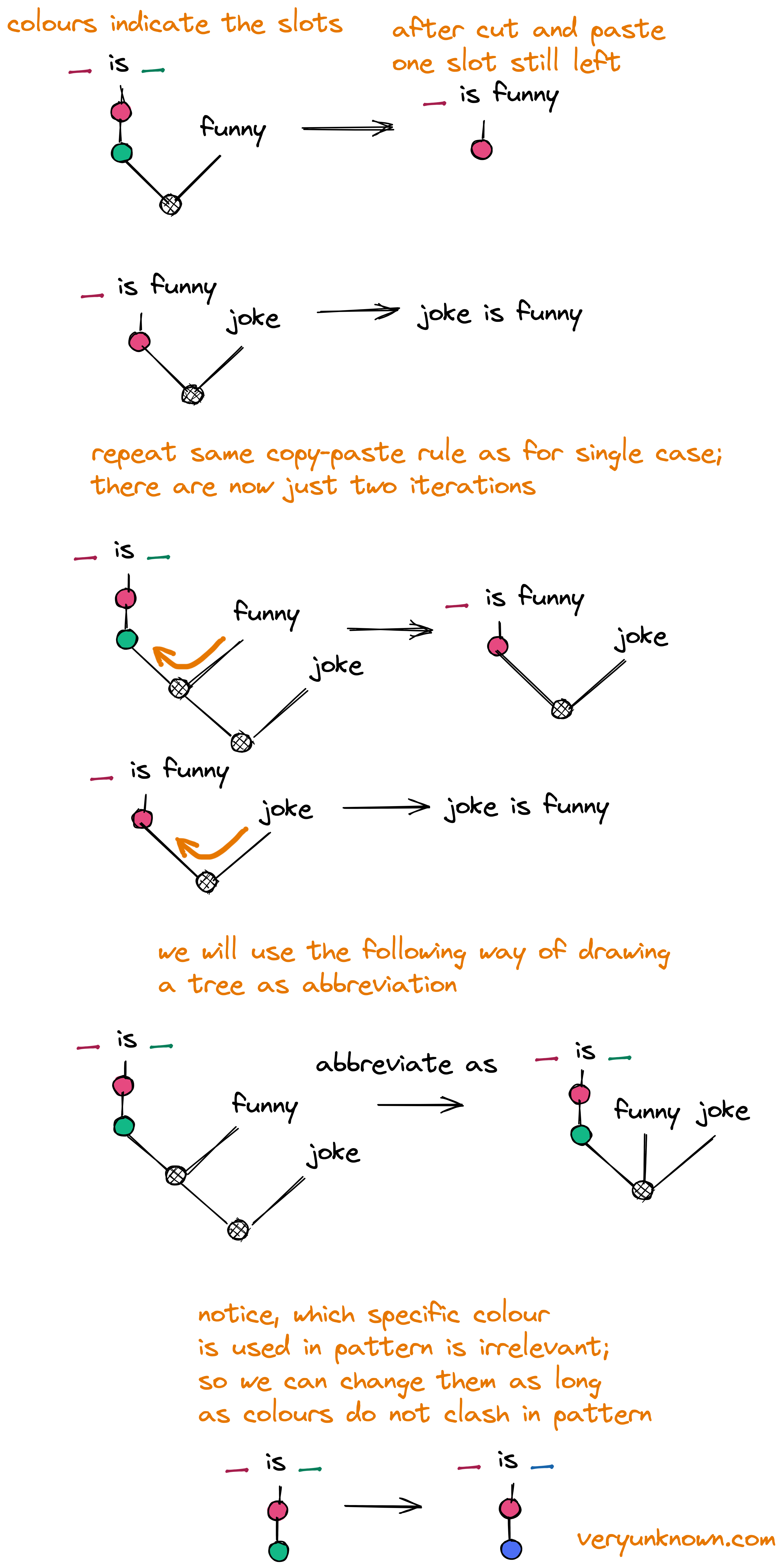
We use colors to distinguish slots, but otherwise all the rules stay the same! Note, how the tree “collapses” every time a colorful dot and black dot are connected with a line! Nothing really changes from single -paste case. We have thus far been putting words on the right side. Can we put other patterns on the right? Yes, we can - we again follow same rules as before. We cut-and-paste the patterns from the right. Lets see Fig 3.
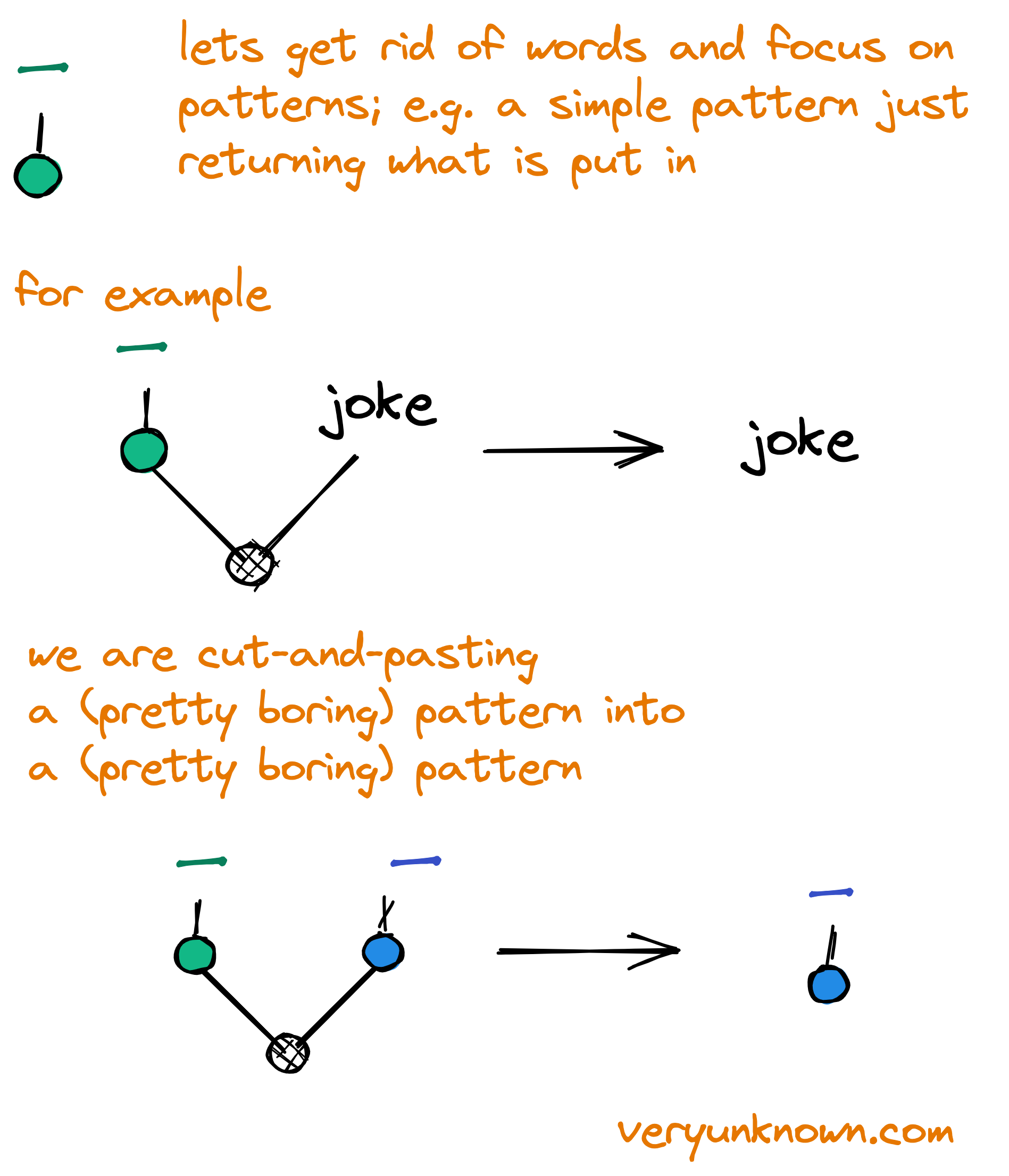
Fig 3. Pattern in pattern
This is it! The Fig 3. seems to be so simple and trivial, that it almost looks nonsensical. But it is not. We have distilled all the rules on which we will build the universe upon!
The rules
Lets summarize the rules:
- There are only patterns
- Specific colours in pattern do not matter; as long as they don’t clash, we can change them (ie, we can recolor)
- We can join patterns. When we see a black circle connected to colourful circle we do “cut and paste” action - cut the from right, paste to left
Basic examples
As initial example we will work on showing how we can start doing some “computing” on values like “true” and “false”. In Fig 4. we will define some patterns. Notice, we are assigning words to patterns, but words themselves do not add anything to what we are doing - they are just shorthand for a tree pattern, so we don’t have to draw bigger trees, and make it easier to read the trees.
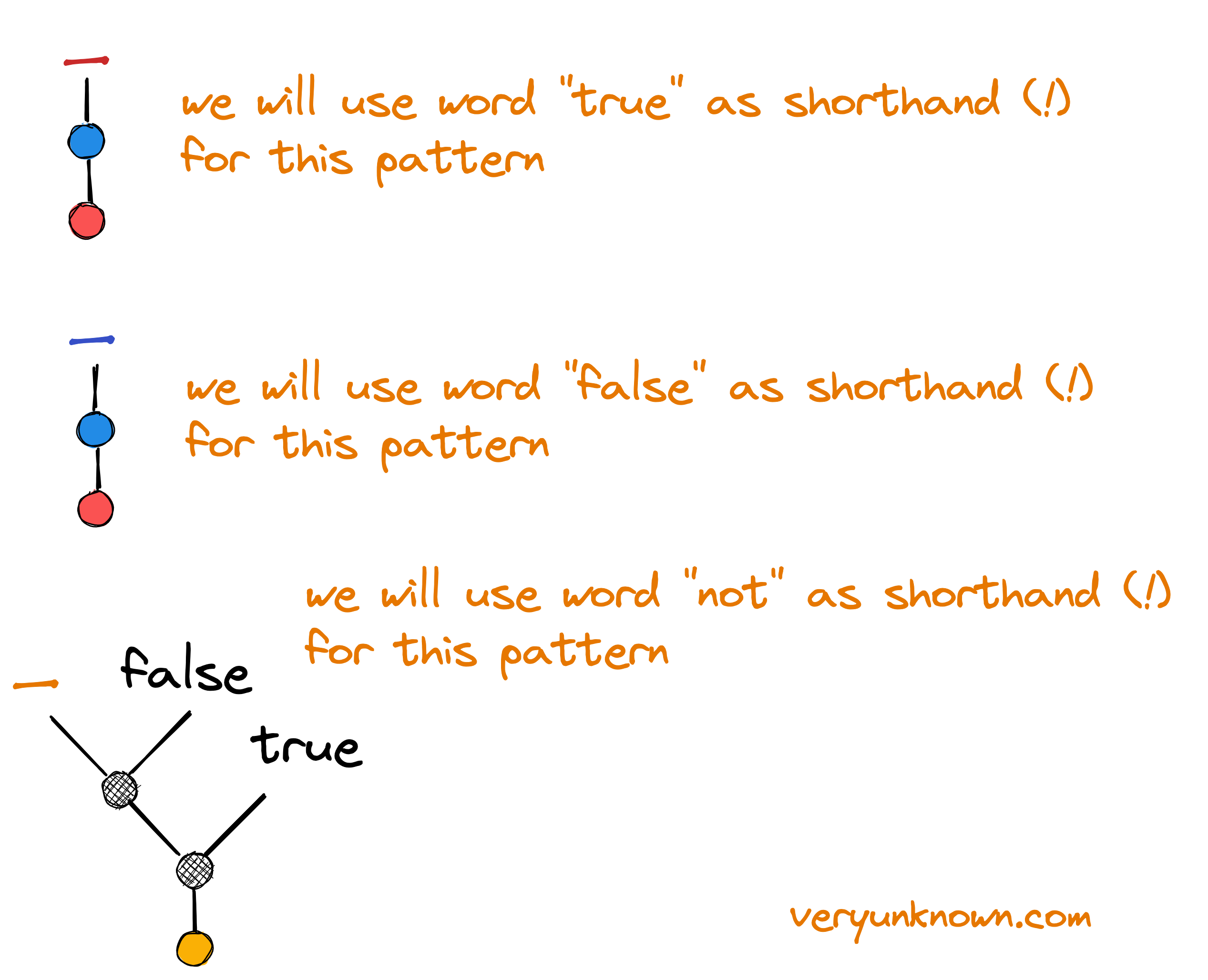
Fig 4. Some example patterns - true/false/not
Why would we choose such patterns and give them such names? To find that out, we need to join them and see what happens!
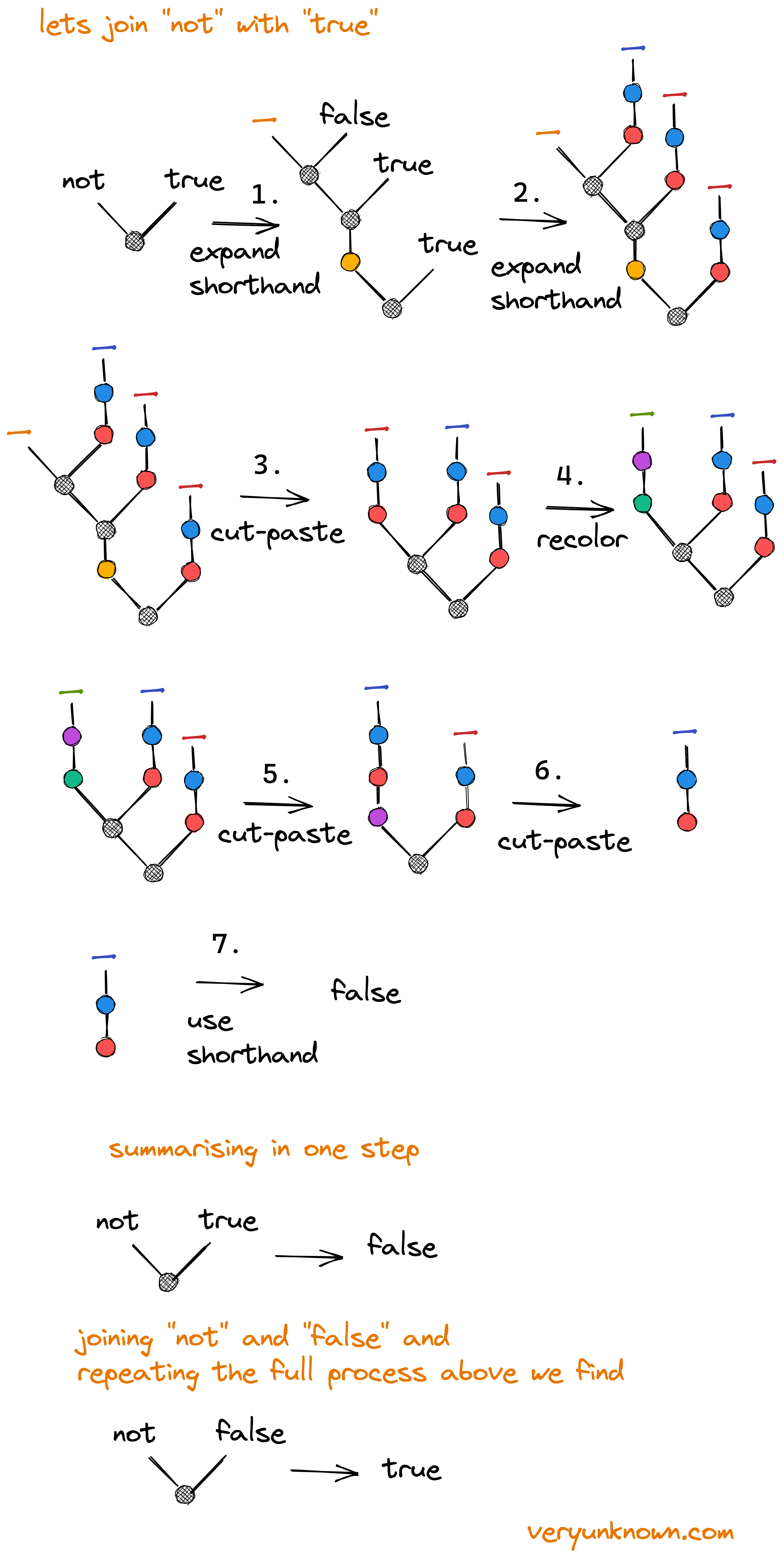
Fig 5. Joining ’not’ with ’true’ and ‘false’
Lets look at Figure 5. and go over the steps in more detail:
- We expand the shorthand “not” to a tree as defined in Figure 4.
- We expand the shorthands “true” and “false” to a tree as defined in Figure 4.
- We note the “join” we can do - the black circle directly connected to the orange circle, and follow the “cut and paste” action as shown in Figure 2. We cut the directly connected pattern on the right side, and paste to the left in the orange slot.
- We note the “join” we can do - the black circle directly connected to the red circle. We notice if we do “cut and paste”, there will be a clash of colours in pattern after the “cut and paste”, so to disambiguate we recolor the pattern - as noted in Figure 2.
- We note the “join” we can do - the black circle directly connected to the green circle, and follow the “cut and paste” action as shown in Figure 2. We cut the right side, and paste to the left.
- We note the “join” we can do - the black circle directly connected to the purple circle, and follow the “cut and paste” action as shown in Figure 2. We cut the right side, and paste to the left. We do the paste to location, where the “purple slot” is. However we don’t see it in the tree so we “paste to nowhere” - in effect the “cut pattern” gets discarded.
- We use shorthand, but in reverse as defined in Figure 4.
We in effect have created two objects “true”/“false” and a function “not” which switches one into another! [1] This is most simple operation from logic we could do. But notice also, that words had no relevance in how we apply the rules. The words are just shorthand for a tree. We could have picked symbol “😊” instead of “true” and symbol “😥” instead of “false” and “change-mood” instead of “not”. Then following the same process as in Fig 5. we would arrive at Fig 6.
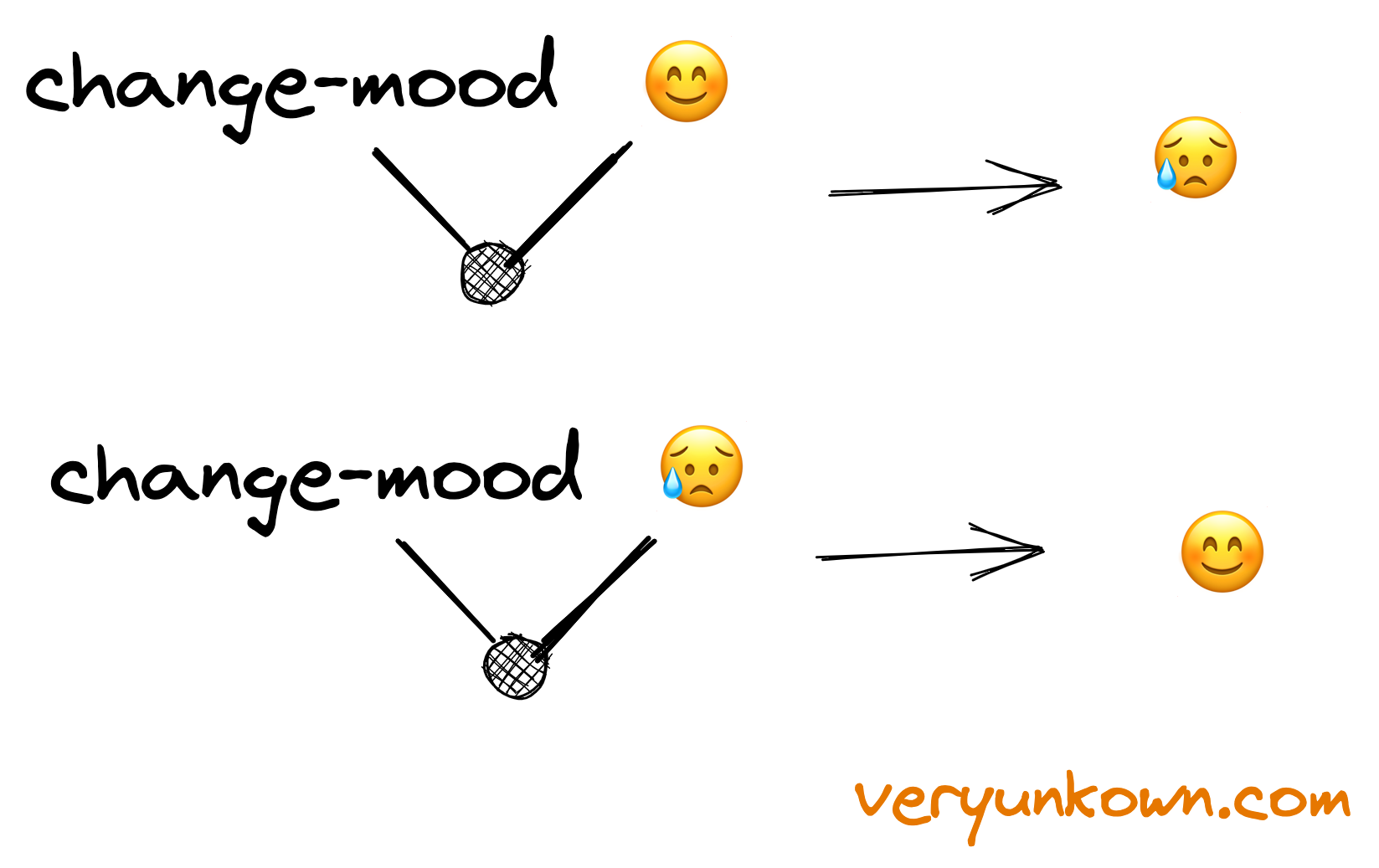
Fig 6. Symbols we use for shorthand are meaningless
“Not” was one of the most simple function we could join with “true” and “false”. We could also define “or” and “and” as well - which, remember, are trees of cut-and-paste patterns. Note, also how there is no real distinction between “function” and “data” in the tree representation - they both are just patterns! In Fig 6. we thought about “😊” and “😥” as data, and “mood-change” as function. But if “😊” / “😥” showed up on the left side of black join dot, they would be functions which could be joined with some “data”.
Building more complex things
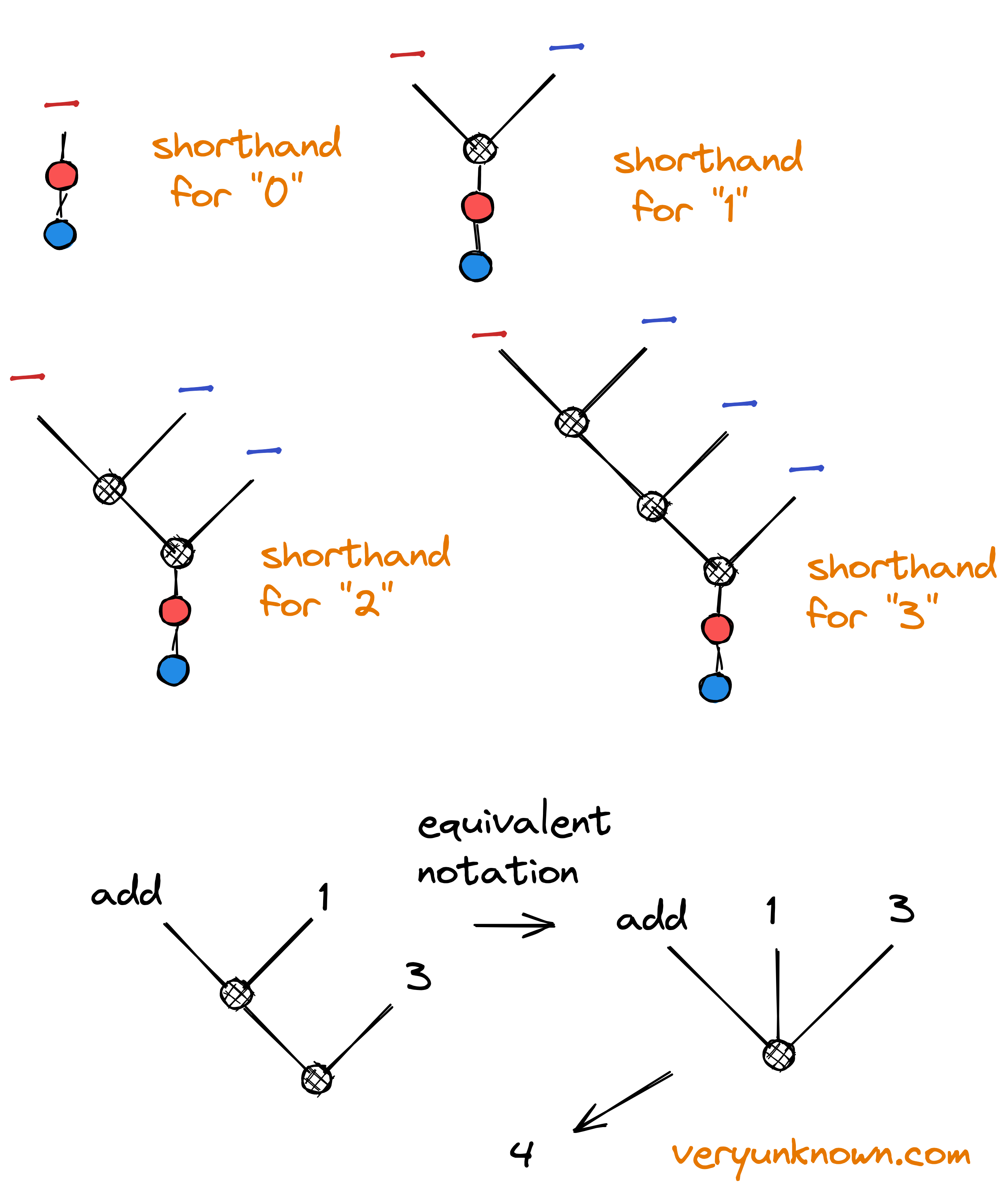
Fig 8. Defining numbers
In previous section we defined one of the most simple things we could think of. However, could we invent more complex things? Answer is a clear yes - with some careful thinking. And the game we would play is exactly like in last section. The more technical term for the game we are playing here with the three basic rules is “lambda calculus”, and was invented by Alonzo Church at start of 20th century. For example, see Fig 8. for how we can define whole positive numbers.

Fig 9. An if statement
Why would we define them in such way? Again the answer is in inventing the other things we can ‘join’ them with. E.g. we can define a pattern “add” in such a way that combining “add” with two numbers yields the expected number (aka tree pattern). We are skipping working through details here, but it would proceed exactly like defining the “not” Fig 4. and then see how it plays out in Fig 5. Evidently we don’t need to stop just at addition, we could define “subtract”, “multiply”, “is-equal”. We could define “if” statement like Fig 9. The key is that we can build up a more complex set of objects and vocabulary, so we can work on higher level than thinking about patterns directly. We can begin to think about “programs” (aka functions) in terms of numbers, and additions, and lists, removing from lists, adding to lists, etc etc. We still build the trees, but we can work on higher abstraction level. Note that under the hood though it always only the 3 rules we outlined in section above! Everything else is just shorthand for said rules.
Repetition
There is one quite special and useful pattern we will look more in detail. When we compute we often want to repeat an action. We can achieve this by utilising a special pattern called “y-combinator”, see Fig 10.
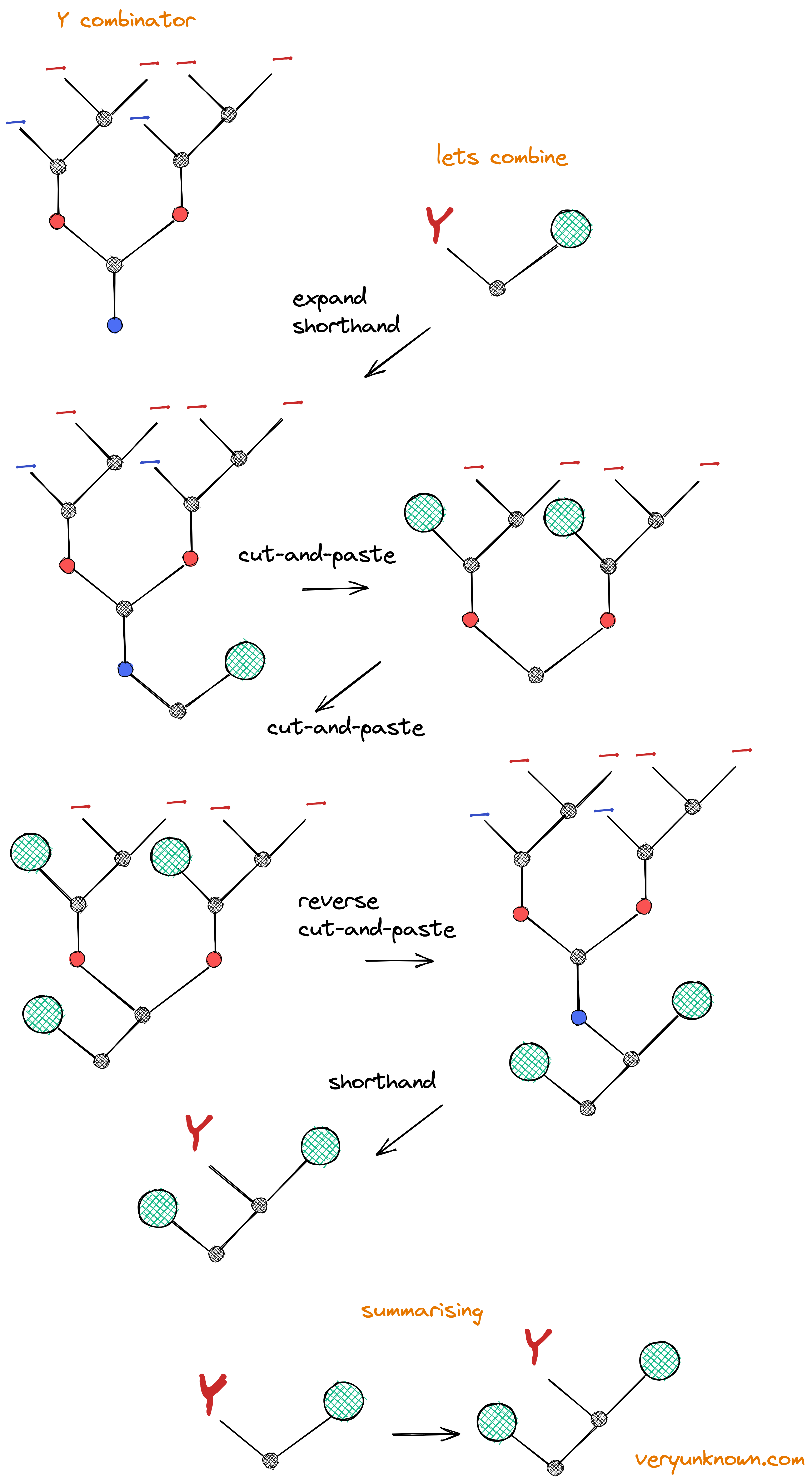
Fig 10. The Y-combinator
Notice how this pattern could keep growing if we used it in some judicious way. That is we can cause a “function” to repeat itself [2]. It’s worth noticing that the tree will not just grow automatically - it depends on what the “green circle” function is in Fig 10 [3]. For example, we could utilize “if” statement in Fig 9. to either keep growing the tree, or chop off the tree growth once it has grown large enough - at which point, the tree will collapse back into final result! We will take advantage of this idea.
Even more complex example
We have explored a range of more complex set of ingredients. Like in physics we started with most basic ingredients - protons and electrons. But now we have built up a bit more complex set of ingredients, like atoms - carbon, oxygen etc, and we can make faster pace doing chemistry. Lets put them together in some more complex example. We will build up a “function” which returns the n-th Fibonacci number. To remind, Fibonacci sequence is list of numbers, where each next one is the sum of previous two: $$ 1, 1, 2, 3, 5, 8, 13, 21, 34, 55, 89, 144 … $$ And we want a function, that e.g. given number “7” (it’s the 7th digit in the list, counting first “1” as 0th digit), it returns “21”. We will use new convention - instead of using colourful circles for cut-and-paste-patterns, we will use colorful words to help follow the meaning of what is being cut-and-pasted where. The general idea how we will approach is, define a function “fibb”, which takes as input “counter”, and two consecutive Fibonacci numbers. Then, if counter is equal to one, we will return second input Fibonacci number as result, otherwise we call “fibb” again, but advance the pair of Fibonacci numbers one step in Fibonacci sequence, and decrement counter by one [4]
Note, that the reader does not need to follow through the Fig 11. It is there just to show how we can keep building more and more complicated structures.
Fig 11. Example of Fibonacci sequence calculation
Simplicity and beauty
We could keep building - create more expressive language, and write more interesting programs. We have atoms, but we could now build molecules. However lets remember, where we started. It has been a very rapid journey. We started with a simple rule at its core for all “computing” - “cutting and pasting” and we have built a “program” for calculating Fibonacci numbers. Programs could get more complicated, but in principle we could create programs for weather simulations, movie animations, chess playing etc., as we mentioned at the start. The “data” would be “today’s weather” and result would be “tomorrow’s weather”, or “current chess board” and result would be “best next move” etc. How come so much complexity can be built up from so little! We have previously found elegance in world of physics in “Inventing special relativity” essay. We have now found it too in world of computing. And curiously, we very tangentially talked that all the symbols have no meaning, but all this symbol shuffling does seem very meaningful! We had a normal sentence “7th element of Fibonacci sequence” and got back “21”. But all we did was symbol shuffling. That leads us to ask, what is the nature of “meaning” if all we do is shuffle meaningless symbols? But it’s a story for another day.
[1] For readers, who are familiar LISP of John McCarthy, we can begin to see how naturally the LISP syntax is beginning to emerge. For example, Fig 5. Could be represented as “(not true)” which returns “false”
[2] We are using “y-combinator” in effect to implement recursion. What is important to notice is - we are implementing recursion without referencing “self”. E.g. in LISP recursion would be implemented as “(def f …. (f …))” or in more imperative languages as “def f(x) { .. f(…) .. }”. In previous definitions of functions they reference themselves - we are explicitly not doing that here! We can achieve “recursion” without self-referencing definitions. This means that we can define functions in terms of finite size trees!
[3] While we have not explicitly emphasized this until now, we do the lowest permissible “join” first, ie. the lowest “color-circle-black-circle” is joined first
[4] In terms of LISP
(def fib [n first second] (
  if (= n 1) second (fib (- n 1) second (+ first second)))
)
(fib 7 1 1)