Why Generative AI?
Generative AI has become quite remarkable in terms of reaching the threshold of quality for human acceptance, e.g. pictures like “Balenciaga Pope” going viral. Generative AI can not only create pictures from a text but also e.g. generate music, create a fleshed-out picture from contours, even create videos, etc. But what exactly is the computer doing when it “generates art”? As we explored in “Lambda calculus visualised”, computers shuffle symbols - not engage in “creativity”. So what does the computer do? In this essay, we will explore generative AI approaches called “diffusion” models (e.g. the “stable diffusion” model). Understanding the inner mechanism of diffusion models can be intimidating as one comes across things like “Stochastic Differential Equations”, “Annealed Langevin dynamics”, etc. So topic can seem quite inaccessible. However, the core mathematical ideas are accessible to any interested reader with a bit of patience - to see how the magic of diffusion based generative AI works. This will be the objective of this essay - not practical implementation, nor a high-level overview, but the exploration of core mathematical ideas of diffusion models which make them work. In particular, we will aim to understand models as introduced in “Deep Unsupervised Learning using Nonequilibrium Thermodynamics” by J. Sohl-Dickstein et al. in 2015.
The main body of the text will focus on core ideas accessible to everyone. However, we will be basically speed-running them - many sub-topics deserve exploration of their own. For the Aficionados the more thorough linking of the “Galton Board model” presented below demands a separate essay, as there will be enough here as is and would demand much more explicit mathematical treatment.
Without further ado, let’s go!
What does a computer generate?
Computers work only with numbers. So what does a computer do when it generates a picture? We should understand how a computer represents a picture. Let’s forget about colors to keep things simpler and consider a greyscale image - as much as the computer is concerned the picture is one long list of numbers, where each number represents the brightness of a pixel. Each row of pixels on the screen is a list of numbers and we can think (loosely) of the whole screen as a concatenated list of pixels for each row. Each list of numbers is unique, and some lists are closer to each other - pictures are more similar visually, but also in the sense that when subtracting two lists of numbers (aka pictures) the resulting differences (loosely) are smaller or bigger. We could keep talking about “lists of numbers” but to keep it a bit more simple, we will switch to just talking about numbers where we think of each number representing a picture.
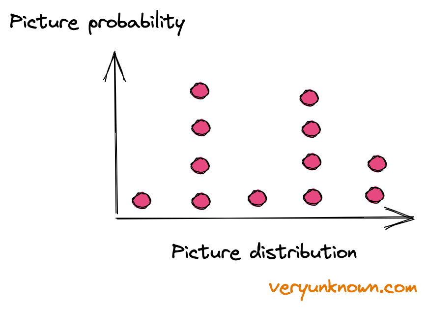
Fig 1. Distribution of pictures
Let’s consider all possible numbers (aka pictures) - most of them would not form a “sensible” picture as deemed by humans. But amongst all the numbers there will be some numbers which we will recognise as sensible. So when we ask the computer to generate a “picture” we ask it in effect to return a number from all possible numbers which are “sensible”. Now some pictures and types of pictures are more probable, while some are less probable, so more precisely computer returns a number proportionally to how likely or unlikely the number (picture) is (see Fig 1). It’s like a computer has biased dice, so generating a picture is the computer “rolling the dice” and reporting the number it sees. The question is - how do we create these “biased digital dice” for computers to roll? And how do we “teach” it the biases given many examples of real pictures?
Galton board as generative AI model
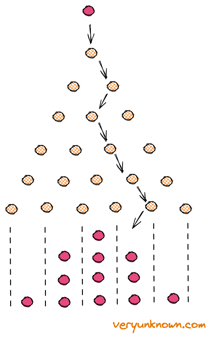
Fig 2. Galton Board
What is a “Galton board”? See Fig 2. It is a mathematical toy. The way it works is that the “orange dots” are pins in the board. Then we drop a ball on the top of the pyramid. At each pin, the solid red ball bounces off in either direction with equal likelihood. And so it keeps tumbling down until it reaches the bottom bucket where we collect all the red balls. If we repeat this many times, the balls at the bottom form a characteristic shape - in the streets known as “normal distribution”. Now is the time for the key idea:
Can we achieve any distribution of balls at the bottom if we adjust each pin to bias bounces just right? The answer is yes! This is the core idea for the “generation” part of the “diffusion” models.
This will be the digital dice - the computer at each step will toss a biased coin, and then take direction left or right depending if the coin flipped head or tails. After repeating the process repeatedly, it will reach the bottom. The generated number is the bucket’s number.
We have the idea for the model, and how to do generation. But we still have the big outstanding question - how do we find the biases for each node?
Training Galton board model
Bottom layer
Fig 3. Galton Board lowest layer Fig 4. Galton Board lowest layer, reverse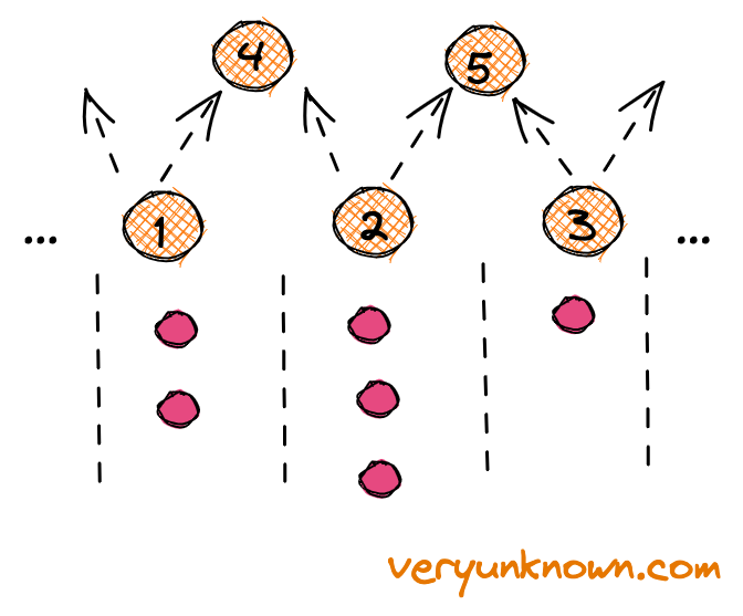
Let us look only at the middle of the very bottom layer in Fig 3. Also, for simplicity of visualization let’s think of a ball traveling through the nodes, not bouncing to the sides of them. We are given a number of balls for each location for the lowest layer (aka our “training data”). We will call them “data balls”. Let’s select one ball at random, and it e.g. happens to be one at location “2”. Let’s take and “kick it” up with equal odds up the left side or the right side - to “4” or “5”. We do such a procedure with all “data balls”. At each higher layer node (ie. “4” and “5”) we keep track of how many times a data ball came from the left side or right side. Now, let’s consider Figure 4. After we have gone through the previous procedure for all our data and collected the “left/right” ratios for nodes “4” and “5” etc we ask the following question - when a ball is falling on node “4” how should we set probabilities of ball bouncing from 4→1 or 4→2 to most “faithfully” represent the data seen at the node “4”?
Let’s think further in terms of odds like more commonly seen in betting. E.g. unfair coin with a double chance of tails would be written as 2:1 (“two to one”) meaning for every time we saw heads we would see two tails. Going back to our question - what would recreate most “faithfully” the seen data examples for 1→4 and 2→4 paths? The intuition is suggesting that the odds should be 1→4:2→4 = 4→1:4→2. E.g. if we saw balls come in from the left 8 times, and from the right 4 times, then we should prefer the left side double the times to the right side.
Feels intuitive. But why? We need to expand on the notion of “faithful representation”. Let’s say we are given the outcome of coin flips and then we are asked - what is the bias of the coin? This is not in itself a question with a unique answer, e.g. we got TTTTT, but a fair coin in principle could have flipped five tails in a row, it’s just unlikely, so we would not think it the best answer. Let’s codify this idea - “the best answer is the biased coin which gives the observed data with maximum probability”. E.g. for TTTTT example then the answer would be a coin that always lands on T. How about HHTTT? We can just calculate the odds of seeing this data for all possible ratios of biased coin, and note the coin with H:T odds giving the observed data with maximum probability would be 2:3. This principle is called “maximum likelihood estimation”, and is the principle we apply in Figure 4.
This is nice! We now have trained a single layer of Galton board as we wanted. But can we start generating our samples? If we have “N” layers, how should we select the nodes on the layer above (aka N-1 layer) to start the downward journey? There is no answer at this point. If we knew the probability of seeing data at note at layer N-1, then we could select the node according to this probability and propagate one layer down. However, we don’t know it, we only know the relative odds for downward paths at each node at N-1 layer. We need something more.
Stacking the layers
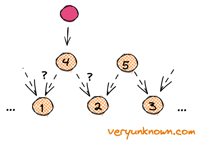
Fig 5. Galton Board lowest layer Fig 6. Stacking the layers from bottom upwards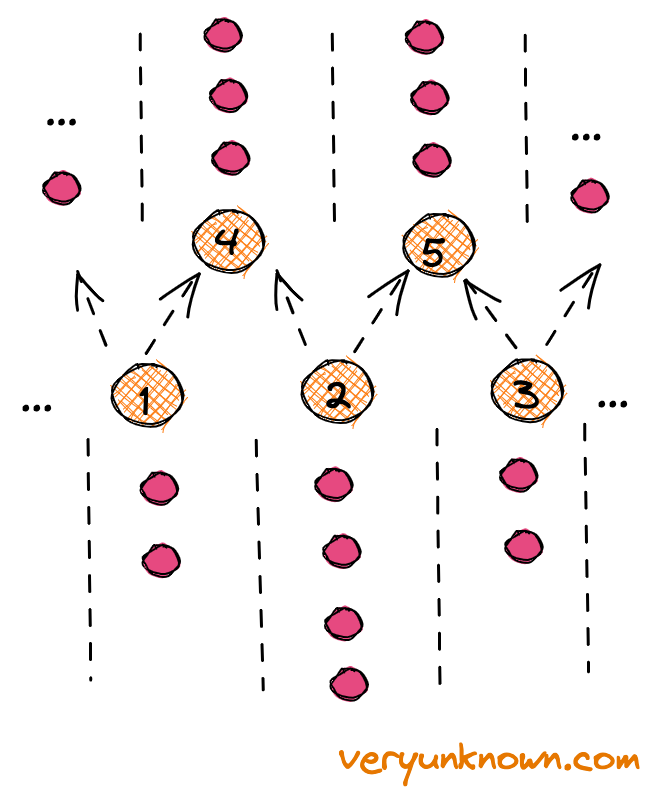
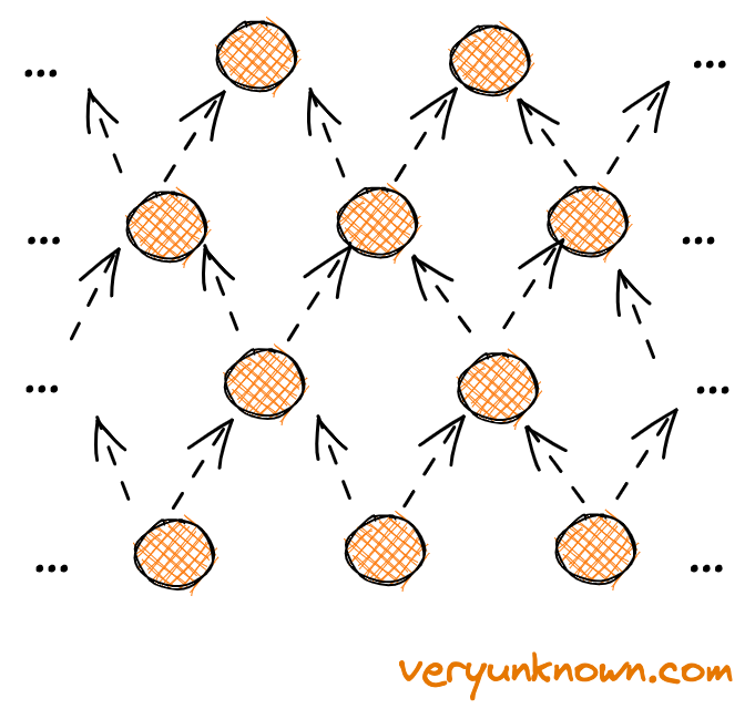
Let’s look at Fig 5. Here is a thing to notice - the higher nodes are mixing balls coming from different locations at lower nodes. Let’s look at an example, e.g. we have 2 data balls at “1”, 4 data balls at “2” and 2 data balls at “3”. How many data balls we will see at “4” and “5”? We will see 3 at both (not to forget from the last section - balls at the lower layer get “kicked up” to the left or right with equal odds). Ie. the number of balls expected to be seen at each location at N-1 layer is “smoothing” out compared with N-th layer. What if we keep stacking? As each layer smoothens the values more and more, then after some number of layers the values will be equal across all the nodes. And now we have the final bit of answer, as now for the generation we can just drop the ball at any top node and let it propagate downwards.
So, to train we have a square shaped model (in contrast to the original toy Galton board), which contains stacked up layers as in Fig 6. As a simplifying assumption, we will consider that our data is on a loop - like a clock, ie. after value 12 comes value 1 (this is not core to our discussion just so we don’t have to worry about having hard edges in Fig 6, so we are connected in a loop). We start at the bottom layer and start kicking the ball upwards, to layer N-1, then to N-2, then to N-3, etc until we reach top layer 0. At each layer, we keep track of left:right ratios (in other words, relative odds of each path). We do this with all our data balls. Then to generate a sample - we drop a ball at the top at any location. That’s that, we have a baby “diffusion” model! We have now seen the answer to the second key question of how to find the biases for each node. To summarise the whole baby model:
We stack our model layers. To train we kick and keep kicking the data balls upwards with equal probability to left and right at each layer to observe data balls at layer-1. We adjust biases to maximize the likelihood of reproducing the observed data balls layer by layer. We will reach a top layer node with equal odds. To generate data we start at any of the top nodes, and propagate downwards randomly, but where each node has its own unique bias
Implementation example
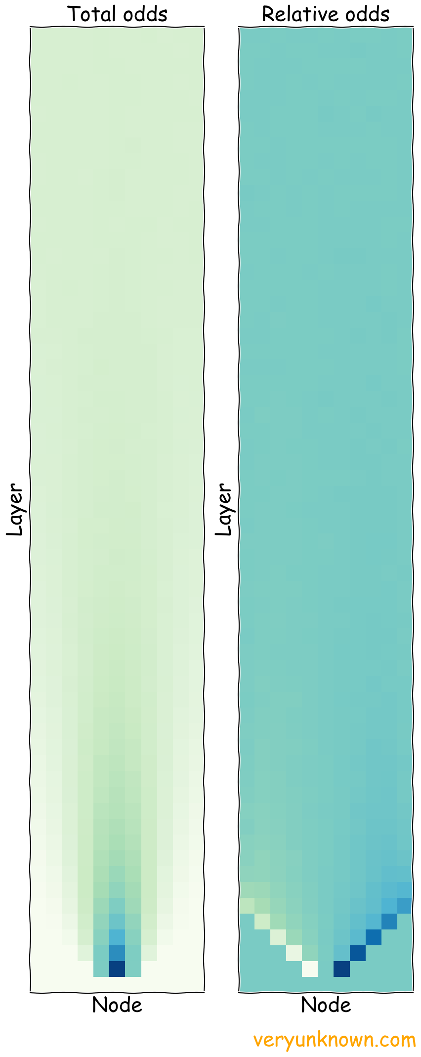
Fig 7. Square galton board model, all training balls
are at 5th node, aka centre
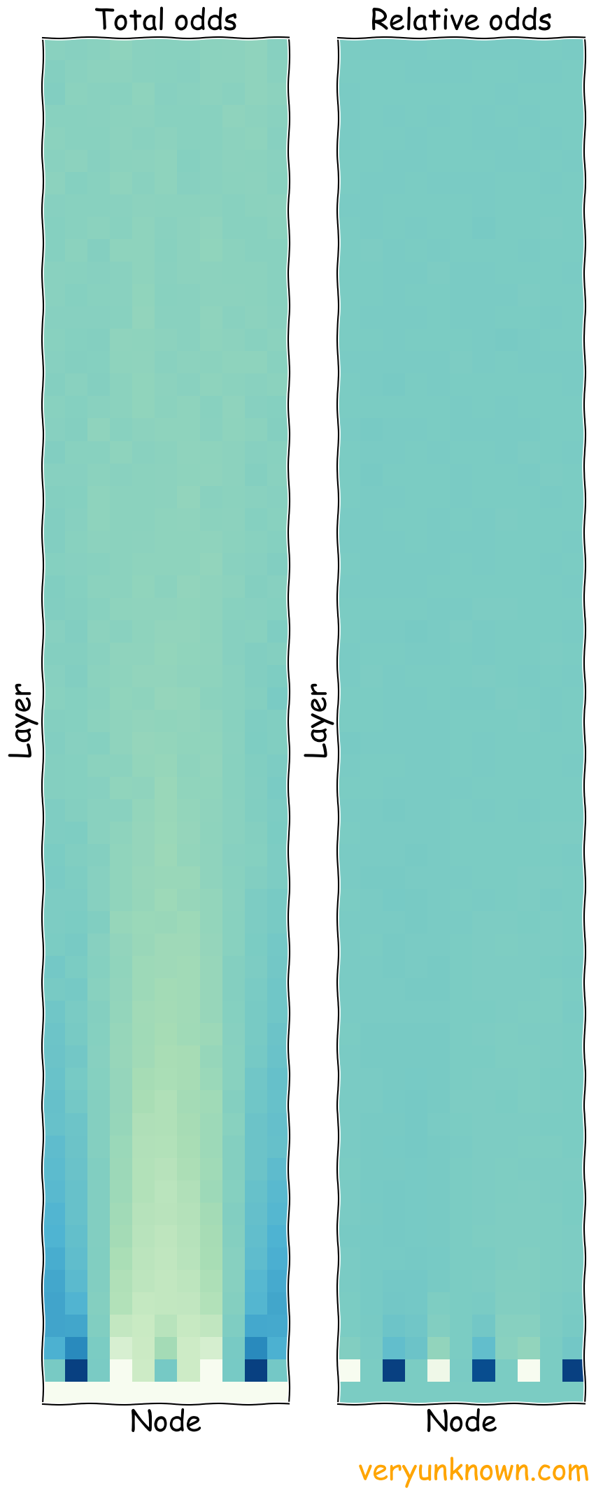
Fig 8. Square galton board model, training balls
are at 5th, 9th and 11th nodes with odds 2:1:2
Now that we have a simple stacked “diffusion” model - we can very much implement it on a computer. Let’s crank the gears - we will use 11 nodes in a layer connected in a loop in Figure 7. It is our “square Galton board” model. We will need to stack up enough layers, that if we have all data balls at a single location at the bottom we get random distribution at the top. We have trained it with the data ball being all in the central 5th node. In the first chart, we plot the odds the node was visited (darker is more likely). While in the right chart, we show relative odds of the node being visited from left or from right (whiter fields mean bias will be more to the right, while dark more biases to the left). Note, that for ease of visualization, we are showing log(left:right) in the relative odds graph.
As expected, at the very bottom the distribution of data balls spread out starting from center, but then even out pretty quickly. The relative odds are as expected too - at the top, we don’t have much bias, while at the bottom of our model, there is a strong bias towards the center. Here we only explored the training bit and the smoothing behavior.
It’s important to note, that what we really care about in the model is the relative odds for each node. We have captured and visualized the total odds for each node for educational purposes. In practice we would in training only attempt to capture relative odds. The total odds are irrelevant for data generation.
How about having a more complicated data distribution? E.g. we will have balls at locations 2, 5, and 9, with relative odds 2:1:2 and zero at all other locations. See Figure 8.
Let’s finally also try to generate some data using the learned relative odds. What distribution of values do we get for the nodes 1-11 at the bottom if we drop many balls at the top? Rounding to 1 decimal point its 2:1:2 for nodes 2, 5, 9 respectively, and 0 odds for the rest as expected.
Towards practicality
We have our basic model of stacked layers. That is the core, but let’s add some more practical considerations. We will neither go through all of them nor go into much detail - but we will sketch some of the ideas towards practical diffusion models.
Broadening jump steps
First, we noticed that distribution gets washed out as we climb upwards, but we needed to add quite a few layers to wash it out completely flat. Could we save ourselves some layers if we increased the size of the step we move sideways? We could indeed. This idea comes by names like aforementioned “annealed Langevin dynamics”.
Drift to the center
Now, previously we worked with a model, where data is on a loop, aka like a clock. However, in more real cases, we wouldn’t assume that. What should we do if we could have any positive or negative value of data? The idea is similar to the “broadening jump” - we adjust our kick-up odds. Instead of always being equal, we bias them towards the “center” nodes by default, so that any data point reaches the central region after passing through the layers upwards. Roughly speaking, the further the data ball is from the center, the bigger bias we apply.
Skipping layers to train
Fig 9. Skipping steps when passing upwards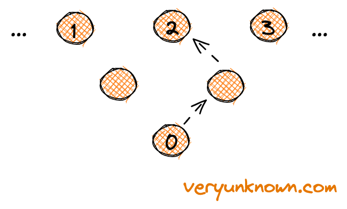
Working with a large number of Nodes and Layers
We normally deal not with discrete numbers, but with smooth sets of numbers. To work with those, we need to in effect consider when the number of nodes tends to infinity, ie. we cover the smooth number line with more and more nodes. This does not affect the concepts but does affect the math. E.g. for the buffs, a quick hint where this would go, we first e.g. notice that our random walk is just a binomial distribution after many steps, which is well approximated by normal distribution after many steps, which has variation \(\sigma \sim \sqrt{n}\). We can note, that instead of thinking of discrete random walks, we can turn to “Kolmogorov forward equation” aka “Fokker–Planck” equation. This then leads us to think of “Kolmogorov backwards equation”, which in turn leads us to consider what \(\sigma\) we should be using (clearly something “small”, but “small” compared to what exactly?). And so we keep going etc etc.
Squashing layers
If we look at the layers in Figure 7 - the adjacent layers look quite similar. Do we really need to have an explicit model for each layer? Currently, we keep track of each layer and each node explicitly. Each adjacent layer looks similar, and adjacent nodes look quite similar too. Could we collapse all of them into a single function, where layer index and node index are parameters? We can indeed. We can deal only with f(node index, layer index, weights)→bias, where “weights” are the model parameters we can tweak instead of counting. We cannot just count anymore to pin down the bias which maximizes the “probability of maximum likelihood” of seen data, but we can still adjust “weights” as dials to find the “maximum likelihood” of seen data.
Generating from text
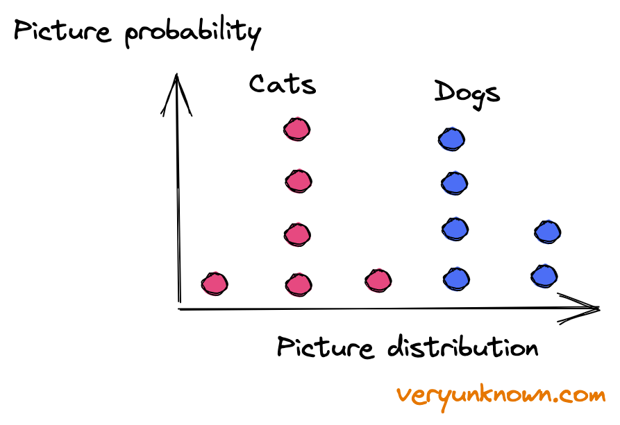
Fig 10. Distribution of pictures of cats and dogs
We are basically done. But common use case is given a word we get a picture. How is that supposed to work in the above description? In the above, we always just generate a picture with adjusted odds to match data. The text conceptually changes little. In effect, our data is split into sets, where each set belongs to a word. Then we generate a network for each. So when we want to generate a sample given a word, we use the right network. As pointed out above though, we have squashed our model into one function f(node, layer, weights)→bias. Each word’s biases are not entirely different. So we could view it as each word adjusts bias from the “all pictures” bias values. So it can be seen as another parameter in our smooth function f(node, layer, weights, word)→bias which we can learn as outlined before based on the “principle of maximum likelihood”.
Where next?
We have dashed very rapidly through. It’s a good time to reflect, sleep and return back to start, as each idea in itself can be revisited in depth as we have elided a lot of details. But we have arrived at the basic shape of a “diffusion model” seen as the “Square Galton Board Tower of Babel” as we set out to do. The next step is to consider when the number of nodes gets very large, ie, what happens when node number \(N\rightarrow\infty\). It adds quite a bit of complication and quite a bit more mathematical complexity. The Aficionados who enjoy talking about e.g. “Kolmogorov forward and backward equations” deserve their own essay outlining in more mathematical detail how the square Galton board model and more regular models relate more precisely. But the basic concepts still stay around and help guide the intuition. Diffusion models are a bit of magic - now we have had a chance to see how the trick is done.