Squaring the Circle
“Squaring the circle” now means chasing the impossible. Originally, it meant something precise: given a circle, construct a square equal in area to it with compass and straightedge alone. It is a tempting problem. Why should the area of a circle not be made square? For over two thousand years, the question remained open. The answer, reached only in 1882 through Ferdinand von Lindemann’s proof, is that it cannot be done with compass and straightedge alone. This essay follows an impossibility proof in full.
We will begin in Greek geometry, then shift perspective. Instead of asking only what figures can be drawn, we ask what numbers can be constructed. That change carries us into algebra, polynomials, and transcendental numbers. A simple-looking puzzle becomes a path through large parts of mathematics.
That is part of the enjoyment. Following the problem leads outward. It teaches new language, reveals hidden structure, and changes the question itself - as good questions can. What first looks like a search for a clever construction becomes a way to see why no such construction can exist.
The prerequisites are modest: basic calculus, high-school polynomials, basic complex numbers, and a rough idea of compass-and-straightedge constructions. The journey is long, but it need not be rushed. Take it at coffee-shop pace. Humanity needed millennia to walk this road for the first time; now we can follow the path too, one step at a time.
Squaring the Circle as a polynomial problem
The journey has two parts: first we translate the geometric problem into a question about numbers and polynomials; then we answer that question. Given a circle of radius \(1\), its area is \(\pi\). A square with the same area must therefore have side length \(\sqrt{\pi}\). So squaring the circle is possible exactly when we can construct a segment of length \(\sqrt{\pi}\). Once that side is drawn, constructing the square itself is routine.
Basic operations of algebra
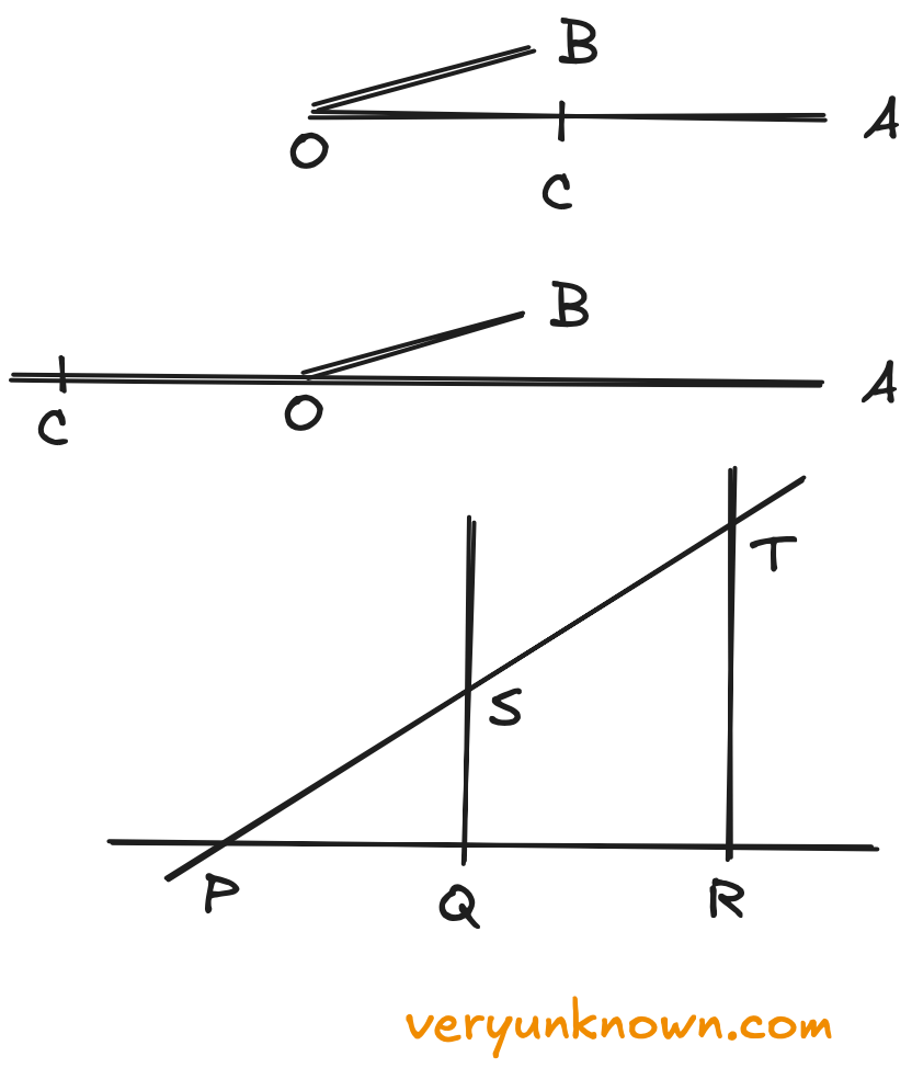
Fig 1. Basic algebra with constructions
To get going, let us first see that straightedge and compass constructions can perform the four basic operations of algebra. Fix a unit segment, and suppose the lengths \(OA\) and \(OB\) have already been constructed:
-
To subtract \(OB\) from \(OA\), use the compass to mark off a copy of \(OB\) along \(OA\). Call the marked point \(C\). Then the leftover segment \(CA\) has length \(OA-OB\).
-
To add, do the opposite: extend the line through \(OA\), mark off a copy of \(OB\) beyond \(A\), and call the marked point \(C\). Then the full segment \(OC\) has length \(OA+OB\).
-
To multiply two constructed lengths \(x\) and \(y\), draw a baseline starting at \(P\). On it, mark \(Q\) so that \(PQ=1\), and farther along mark \(R\) so that \(PR=y\). Erect perpendiculars at \(Q\) and \(R\) (how to construct them is Proposition 11 in Euclid’s Elements). On the perpendicular at \(Q\), mark \(S\) so that \(QS=x\). Now draw the line \(PS\), and let it meet the perpendicular at \(R\) at a point \(T\). The right triangles \(PQS\) and \(PRT\) are similar, so $$ \frac{RT}{QS}=\frac{PR}{PQ}=\frac{y}{1} $$ Since \(QS=x\), this gives \(RT=xy\). So the length \(xy\) is constructible.
-
Division uses the same picture and the same general idea as multiplication, but in reverse.
These are the standard constructible-number operations: addition and subtraction come from copying lengths on a line; multiplication and division come from similar triangles.
Why only algebra and square roots appear
Now comes the key change of viewpoint. Moving from geometric drawings to coordinates may feel like a sudden change of subject, but coordinates simply record exactly what each construction has produced. A straightedge-and-compass construction creates points, and once we fix a starting point and a unit segment, every point can be described by coordinates. So the real question becomes: what kinds of new coordinates can appear when we draw lines and circles?
We already know that rational numbers can be constructed. Starting from a unit segment, we can add, subtract, multiply, and divide constructed lengths, so every rational number is available to us. The next question is whether intersections of lines and circles can introduce anything more. A new point can only appear as the intersection of two already constructed objects. There are only three possible cases.
-
For a line meeting a line, we solve two linear equations: $$ ax+by=c,\qquad dx+ey=f $$ Solving gives $$ x=\frac{ce-bf}{ae-bd},\qquad y=\frac{af-cd}{ae-bd}, $$ assuming the lines are not parallel. These formulas use only \(+,-,\times,\div\), so line-line intersections do not give us any new kind of number.
-
For a line meeting a circle, we solve $$ ax+by=c,\qquad (x-p)^2+(y-q)^2=r^2 $$ The line lets us express one variable in terms of the other. Substituting into the circle gives a quadratic equation: $$ Au^2+Bu+C=0 $$ Its solutions are $$ u=\frac{-B\pm\sqrt{B^2-4AC}}{2A} $$ So line-circle intersections introduce one new operation: taking a square root.
-
For a circle meeting a circle, we solve $$ (x-p)^2+(y-q)^2=r^2,\qquad (x-m)^2+(y-n)^2=s^2 $$ Subtracting the two equations cancels the \(x^2\) and \(y^2\) terms, leaving a linear equation: $$ 2(m-p)x+2(n-q)y=r^2-s^2+m^2+n^2-p^2-q^2 $$ We can see this as another instance of line meeting a circle, so nothing new here.
So every step in a straightedge-and-compass construction uses only the four basic operations and, when a circle is involved, a square root. No other kind of number can show up. In other words, every coordinate you can construct comes from repeatedly using those same five operations.
Turning constructed numbers into polynomial roots
This has a powerful consequence: every constructible number is algebraic. A number is called algebraic if it is a root of some non-zero polynomial with integer coefficients. In plain language, if a number \(x\) can be built from rational numbers using basic algebra operations and square roots, then \(x\) satisfies some polynomial equation with integer coefficients.
An example makes it easy to see why it is so. Suppose \(x=\sqrt{1+\sqrt{2/3}}\). Then \(x^2=1+\sqrt{2/3}\), so \(x^2-1=\sqrt{2/3}\). Squaring again gives \((x^2-1)^2=2/3\). Multiplying by \(3\), we get \(3(x^2-1)^2=2\). Expanding, \(3x^4-6x^2+3=2\), and therefore \(3x^4-6x^2+1=0\). So \(x=\sqrt{1+\sqrt{2/3}}\) is not just a nested expression: it is also a root of the polynomial equation \(3x^4-6x^2+1=0\).
This is the bridge we need: if we can show that a number is not the root of any polynomial equation with integer coefficients, then it cannot be constructed.
Proof that \(\pi\) is a transcendental number
Non-algebraic numbers are called transcendental numbers. If we could construct a segment of length \(\sqrt{\pi}\), then the multiplication construction above would give us a segment of length \(\pi\). Thus it is enough to show that \(\pi\) is transcendental and therefore not constructible. At a high level, the proof will assume that \(\pi\) is algebraic and derive a contradiction, so the assumption must have been false.
Polynomial prerequisites
Before diving into the proof, we will quickly go through a few prerequisites on polynomials.
If \(r\) is algebraic, then so is \(ir\)
Suppose \(r\) is algebraic. Then there is a nonzero polynomial \(p(z)\) with rational coefficients such that \(p(r)=0\). Define \(Q(z)=p(iz)p(-iz)\), and plug in \(z=ir\): $$ Q(ir)=p(i(ir))p(-i(ir))=p(-r)p(r)=p(-r)\cdot 0=0 $$ So \(ir\) is a root of \(Q(z)\). Now check that \(Q(z)\) has rational coefficients. Split \(p(z)\) into its even-power and odd-power parts: \(p(z)=A(z^2)+zB(z^2)\), where \(A\) and \(B\) have rational coefficients. Then $$ Q(z)=\bigl(A(-z^2)+izB(-z^2)\bigr)\bigl(A(-z^2)-izB(-z^2)\bigr) =A(-z^2)^2+z^2B(-z^2)^2 $$ This expression has only rational coefficients, and \(Q(z)\) is nonzero because it is a product of two nonzero polynomials. Therefore, if \(r\) is algebraic, then so is \(ir\).
Vieta’s formulas
Start with two roots, \(r_1\) and \(r_2\). The simplest polynomial with these roots is \((z-r_1)(z-r_2)\). This is monic, meaning its leading coefficient is \(1\). Expanding gives \((z-r_1)(z-r_2)=z^2-(r_1+r_2)z+r_1r_2.\) One should take note of the relationship between the roots and the polynomial coefficients. Let us try with three roots: \((z-r_1)(z-r_2)(z-r_3)=z^3-(r_1+r_2+r_3)z^2+(r_1r_2+r_1r_3+r_2r_3)z-r_1r_2r_3.\)
The general pattern is this: if \(r_1,\ldots,r_n\) are the roots of a monic polynomial \(z^n+c_{n-1}z^{n-1}+c_{n-2}z^{n-2}+\cdots+c_1z+c_0\), then its coefficients are related to the roots by \(c_{n-1}=-(r_1+\cdots+r_n)\), \(c_{n-2}=\sum_{1\leq i\lt j\leq n} r_ir_j\), \(c_{n-3}=-\sum_{1\leq i\lt j\lt k\leq n} r_ir_jr_k\), and so on, until \(c_0=(-1)^nr_1r_2\cdots r_n\).
If the polynomial is not monic, nothing serious changes. Suppose the polynomial is \(c_nz^n+c_{n-1}z^{n-1}+\cdots+c_0\), with leading coefficient \(c_n\). Dividing by \(c_n\) makes it monic, so the same relationships hold with each coefficient divided by \(c_n\). For example, the sum of the roots is \(-c_{n-1}/c_n\), the pair-product sum is \(c_{n-2}/c_n\), etc. This is Vieta’s formula.
The Fundamental Theorem of Symmetric Polynomials
The root-combinations that appear in Vieta’s theorem have a name: they are called elementary symmetric polynomials. For roots \(r_1,r_2,r_3\), they are \(r_1+r_2+r_3\), then \(r_1r_2+r_1r_3+r_2r_3\), then \(r_1r_2r_3\). They are “symmetric” because nothing changes if we reorder the roots. But in what sense are they elementary? For example, \(r_1^3+r_2^3+r_3^3\) is also symmetric, but it is not one of these basic pieces. The Fundamental Theorem of Symmetric Polynomials says that every symmetric polynomial can be rewritten using only the elementary symmetric polynomials.
Here is the idea in one concrete case. Let \(s_1=r_1+r_2+r_3\), \(s_2=r_1r_2+r_1r_3+r_2r_3\), and \(s_3=r_1r_2r_3\). Then \( r_1^3+r_2^3+r_3^3=s_1^3-3s_1s_2+3s_3.\) So even though \(r_1^3+r_2^3+r_3^3\) looks different from Vieta’s root-combinations, it can still be rebuilt from them.
The proof of the theorem is basically an algorithm: keep rewriting the largest remaining terms of a symmetric polynomial using elementary symmetric polynomials. We will not dwell on that algorithm here, since we only need the result, not the machinery behind it.
Subset sums of roots give rational polynomials
Suppose \(\alpha_1,\alpha_2,\alpha_3\) are the roots of a polynomial with rational coefficients. The claim is that sums of these roots are algebraic too: they themselves occur as roots of some polynomial with rational coefficients. Let us see why with an example. Consider all the pairwise sums \(\alpha_1+\alpha_2\), \(\alpha_1+\alpha_3\), and \(\alpha_2+\alpha_3\). Build the polynomial whose roots are these sums: \(H(x)=(x-(\alpha_1+\alpha_2))(x-(\alpha_1+\alpha_3))(x-(\alpha_2+\alpha_3))\).
When expanded, the coefficients of \(H(x)\) are symmetric in \(\alpha_1,\alpha_2,\alpha_3\): if we swap the names of the \(\alpha\)’s, we only rearrange the same three factors, so the product remains the same. By the Fundamental Theorem of Symmetric Polynomials, the coefficients of \(H(x)\) can be rewritten using the elementary symmetric polynomials in \(\alpha_1,\alpha_2,\alpha_3\). By Vieta’s theorem, those elementary symmetric polynomials are rational numbers, because the original polynomial has rational coefficients. Therefore \(H(x)\) has rational coefficients. The same idea works in general, no matter how many roots there are or how many roots we add at a time.
Proof that \(\pi\) is transcendental
We have already walked quite a journey, and we are finally ready to embark on the core proof. We will basically follow the proof outlined in Galois Theory by I. Stewart, but we will slow it down, expand the steps, and proceed at a slightly more relaxed pace. At a high level, the proof has three steps:
- Set up an equality using calculus, where both sides must be equal.
- Show that one side of the equation must be a nonzero integer, assuming \(\pi\) is algebraic.
- Show, using basic calculus, that the other side of the equation must have absolute value less than one.
This gives a contradiction, so \(\pi\) is transcendental, and the classical problem of squaring the circle is impossible.
Set up the \(\beta\)’s and their polynomial
Assume, for contradiction, that \(\pi\) is algebraic. By the earlier fact that if \(\pi\) is algebraic, then \(i\pi\) is also algebraic, there is a polynomial \(q(x)\) with rational coefficients whose roots are \(\alpha_1,\alpha_2,\dots,\alpha_n\), with \(\alpha_1=i\pi\). Using Euler’s identity \(e^{i\pi}+1=0\), we get \(e^{\alpha_1}+1=0\), and therefore $$ (e^{\alpha_1}+1)(e^{\alpha_2}+1)\cdots(e^{\alpha_n}+1)=0, $$ as the first factor is already zero. Now we expand this product. A small example shows the pattern: $$ \begin{gathered} (1+e^{\alpha_1})(1+e^{\alpha_2})(1+e^{\alpha_3}) \\ = 1+e^{\alpha_1}+e^{\alpha_2}+e^{\alpha_3} +e^{\alpha_1+\alpha_2} +e^{\alpha_1+\alpha_3} +e^{\alpha_2+\alpha_3} +e^{\alpha_1+\alpha_2+\alpha_3} \end{gathered} $$
So the exponents that appear are all the subset sums of the roots \(\alpha_1,\dots,\alpha_n\). The expansion always includes the term \(1\), and other subset sums might also equal zero. Each of those terms gives \(e^0=1\). Let \(k\) be the total contribution of all these \(1\)’s. Since the expansion always includes the term \(1\), we have \(k>0\). Now collect the nonzero exponential terms into one list, and call their exponents \(\beta_1,\beta_2,\dots,\beta_r\). Then the expanded product has the form $$ e^{\beta_1}+e^{\beta_2}+\cdots+e^{\beta_r}+k=0 $$ Let us park this equation; we will use it later. Now we build a polynomial whose roots are exactly \(\beta_1,\dots,\beta_r\). First look at the two-root sums polynomial: $$ \prod_{1\le i\lt j\le n}\left(x-(\alpha_i+\alpha_j)\right) $$ By the earlier subset-sum result, this polynomial has rational coefficients. If one of the sums \(\alpha_i+\alpha_j\) is zero, then the corresponding factor is just \(x\), and since the \(\beta\)’s only include nonzero exponents, we remove any such \(x\)-factors. Call the remaining polynomial \(\theta_2(x)\). Its roots are exactly the nonzero two-root sums.
The same pattern gives \(\theta_1(x)\) for the nonzero one-root sums, \(\theta_3(x)\) for the nonzero three-root sums, and so on, up to \(\theta_n(x)\). Each of these polynomials still has rational coefficients. Now multiply all these polynomials: $$ \theta(x)=\theta_1(x)\theta_2(x)\cdots\theta_n(x) $$ \(\theta(x)\) has rational coefficients and roots \(\beta_1,\dots,\beta_r\). Finally, multiply \(\theta(x)\) by a suitable integer so that all its coefficients become integers.
Write \(\theta(x)=cx^r+c_1x^{r-1}+\cdots+c_r\). Since zero is not one of the roots of this final polynomial, the constant term is nonzero, so \(c_r\neq 0\).
Define the magic polynomial
For now, choose a prime \(p\). Later we will choose \(p\) carefully, but at this point it is just a prime number. Set \(s=rp-1\), and define $$ f(x)=\frac{c^s x^{p-1}\theta(x)^p}{(p-1)!} $$
This is a carefully engineered polynomial. It is fair to wonder how anyone first thought of it, but that historical question would take us too far from the proof itself. For now, we will stay on the main road. As we proceed, the purpose of its individual pieces will become clearer. The proof of the pudding, as the saying goes, is in the eating.
The equality
Let us also define a related polynomial
$$ F(x)=f(x)+f^{\prime}(x)+f^{\prime\prime}(x)+\cdots+f^{(s+p+r-1)}(x) $$
When we differentiate \(F(x)\), the terms shift one step: \(f(x)\) becomes \(f^{\prime}(x)\), \(f^{\prime}(x)\) becomes \(f^{\prime\prime}(x)\), and so on. Since \(f(x)\) is a polynomial, the extra high derivative at the end is zero. So when we subtract \(F(x)\) from \(F^{\prime}(x)\), all the derivative terms cancel and only \(-f(x)\) remains. Thus
$$ F^{\prime}(x)-F(x)=-f(x) $$
Now fix a value of \(x\). Later \(x\) will be one of the \(\beta_j\)’s, so \(x\) may be complex. To avoid any complex path-integral language, we only use the real variable \(\lambda\), where \(0\le \lambda\le 1\). Think of \(x\) as a constant. By the ordinary chain rule,
$$ \frac{d}{d\lambda}\left(e^{-\lambda x}F(\lambda x)\right) = -xe^{-\lambda x}F(\lambda x) + xe^{-\lambda x}F^{\prime}(\lambda x) $$
Using \(F^{\prime}-F=-f\), this becomes
$$ \frac{d}{d\lambda}\left(e^{-\lambda x}F(\lambda x)\right) = xe^{-\lambda x}\bigl(F^{\prime}(\lambda x)-F(\lambda x)\bigr) = -xe^{-\lambda x}f(\lambda x) $$
Integrating from \(\lambda=0\) to \(\lambda=1\), we get
$$ e^{-x}F(x)-F(0) = -x\int_0^1 e^{-\lambda x}f(\lambda x)\,d\lambda $$
Multiplying by \(e^x\), we get
$$ F(x)-e^xF(0) = -x\int_0^1 e^{(1-\lambda)x}f(\lambda x)\,d\lambda $$
Now plug in \(x=\beta_j\), and sum over \(j=1,\dots,r\). This gives
$$ \sum_{j=1}^r F(\beta_j) - \left(\sum_{j=1}^r e^{\beta_j}\right)F(0) = -\sum_{j=1}^r \beta_j \int_0^1 e^{(1-\lambda)\beta_j}f(\lambda\beta_j)\,d\lambda $$
But from the previous section, \(e^{\beta_1}+\cdots+e^{\beta_r}+k=0\), so \(\sum_{j=1}^r e^{\beta_j}=-k\). Therefore
$$ \sum_{j=1}^r F(\beta_j)+kF(0) = -\sum_{j=1}^r \beta_j \int_0^1 e^{(1-\lambda)\beta_j}f(\lambda\beta_j)\,d\lambda $$
The rest of the proof compares the two sides.
Estimate the right side
The right side of the equality after plugging in \(f\) is
$$ R_p = -\sum_{j=1}^r \beta_j \int_0^1 e^{(1-\lambda)\beta_j} \frac{c^s(\lambda\beta_j)^{p-1}\theta(\lambda\beta_j)^p}{(p-1)!} \,d\lambda $$
We want to show that by choosing the prime \(p\) large enough, we can make \(|R_p|\lt 1\). We can find fixed bounds \(|\beta_j|\le L\), \(|\theta(\lambda\beta_j)|\le M\), and \(|e^{(1-\lambda)\beta_j}|\le B\). These bounds do not depend on \(p\). Taking absolute values and using these bounds gives
$$ |R_p| \le \sum_{j=1}^r L \int_0^1 \frac{ B |c|^s(\lambda L)^{p-1}M^p }{(p-1)!} \,d\lambda \le \sum_{j=1}^r \frac{ B|c|^sL^pM^p }{(p-1)!} \int_0^1 \lambda^{p-1}\,d\lambda $$
Since \(\int_0^1 \lambda^{p-1}\,d\lambda=1/p\), summing and using \(s=rp-1\) gives
$$ |R_p| \le \frac{rB|c|^sL^pM^p}{p!} \le \frac{rB|c|^{rp-1}L^pM^p}{p!} = \frac{rB}{|c|} \frac{\bigl(|c|^rLM\bigr)^p}{p!} $$
Set \(A=|c|^rLM\) and \(C=rB/|c|\). Then our bound is simply
$$ |R_p|\le C\frac{A^p}{p!} $$
The numbers \(A\) and \(C\) are fixed - only \(p\) changes. The factor \(p!\) grows much faster than \(A^p\). To see this, let \(a_p=A^p/p!\). Then
$$ \frac{a_{p+1}}{a_p}=\frac{A}{p+1} $$
Once \(p\) is large enough, this ratio is less than \(1/2\). So the bound keeps shrinking and can be made smaller than \(1\). Since primes can be chosen as large as we like, choose a prime \(p\) such that
$$ |R_p|\lt 1 $$
The left side is a nonzero integer
The left side is
$$ L_p=\sum_{j=1}^rF(\beta_j)+kF(0) $$
We will show that, for all sufficiently large prime \(p\), this is a nonzero integer. Since \(F=f+f^{\prime}+f^{\prime\prime}+\cdots\), we will need to understand the derivatives of \(f\) at the points \(\beta_1,\dots,\beta_r\) and at \(0\).
The sum of F at the roots
This will probably be the most fiddly portion of the proof. First consider \(t\lt p\). Write \(f(x)=u(x)\theta(x)^p\), where \(u(x)\) is everything in \(f(x)\) except the factor \(\theta(x)^p\). Since \(\theta(\beta_j)=0\), we immediately get \(f(\beta_j)=0\). For the first derivative, \(f^{\prime}(x)=u^{\prime}(x)\theta(x)^p+u(x)p\theta(x)^{p-1}\theta^{\prime}(x)\). Both terms still contain a factor of \(\theta(x)\), so \(f^{\prime}(\beta_j)=0\). The same pattern continues with higher derivatives. Therefore \(f^{(t)}(\beta_j)=0\) for \(t\lt p\).
Now consider \(t\ge p\). Let \(H(x)=x^{p-1}\theta(x)^p\), so \(f(x)=c^sH(x)/(p-1)!\). Since \(\theta(x)\) has integer coefficients, \(H(x)\) also has integer coefficients. Let us look at any term \(a_mx^m\) of \(H(x)\) that survives after \(t\) derivatives, so \(m\ge t\). Its \(t\)-th derivative is
$$ a_m\frac{m!}{(m-t)!}x^{m-t} $$
After dividing by \((p-1)!\), the coefficient becomes
$$ a_m\frac{m!}{(m-t)!(p-1)!} = a_m\frac{m!}{t!(m-t)!}\cdot \frac{t!}{(p-1)!} $$
The first fraction is a whole number: it is the number of ways to choose \(t\) objects from \(m\) objects. Since \(t\ge p\), the second fraction is
$$ \frac{t!}{(p-1)!}=p(p+1)\cdots t, $$
which is divisible by \(p\). Therefore \(H^{(t)}(x)/(p-1)!\) has integer coefficients, all divisible by \(p\). In other words, after dividing every coefficient by \(p\), we still have a polynomial with integer coefficients - call that polynomial \(P_t(x)\), so
$$ \frac{H^{(t)}(x)}{(p-1)!}=pP_t(x) $$
Differentiating \(f(x)\) gives
$$ f^{(t)}(x)=c^s\frac{H^{(t)}(x)}{(p-1)!}=pc^sP_t(x), $$
Here \(P_t(x)\) has integer coefficients. Recall that \(H(x)=x^{p-1}\theta(x)^p\). Since \(\theta(x)\) has degree \(r\), the degree of \(H(x)\) is \((p-1)+rp=s+p\). Taking \(t\) derivatives lowers the degree by \(t\), and here \(t\ge p\), so the degree of \(P_t(x)\) is at most \(s\). So we can write \(P_t(x)=b_0+b_1x+\cdots+b_sx^s\), where the \(b_i\)’s are integers.
Now sum over \(\beta_1,\dots,\beta_r\):
$$ \sum_{j=1}^r f^{(t)}(\beta_j) = pc^s\sum_{j=1}^r P_t(\beta_j) $$
Expanding \(P_t(\beta_j)\) gives
$$ \sum_{j=1}^r P_t(\beta_j) = \sum_{j=1}^r \left(b_0+b_1\beta_j+b_2\beta_j^2+\cdots+b_s\beta_j^s\right) $$
Rearranging,
$$ \sum_{j=1}^r P_t(\beta_j) = b_0r +b_1\sum_{j=1}^r\beta_j +b_2\sum_{j=1}^r\beta_j^2 +\cdots +b_s\sum_{j=1}^r\beta_j^s $$
Each sum \(\sum_{j=1}^r\beta_j^m\) is symmetric in the roots \(\beta_1,\dots,\beta_r\). By the Fundamental Theorem of Symmetric Polynomials, it can be rewritten using the elementary symmetric sums of the \(\beta\)’s. By Vieta’s formulas, each elementary symmetric sum of the \(\beta\)’s is, up to sign, one of the integer coefficients of \(\theta\) divided by the leading coefficient \(c\). When the power sum \(\sum_j\beta_j^m\) is rewritten using these elementary symmetric sums, the worst possible denominator is \(c^m\), and since \(m\le s\), the factor \(c^s\) in our expression clears all these denominators. Hence \(c^s\sum_{j=1}^r P_t(\beta_j) \) is an integer. Therefore
$$ \sum_{j=1}^r f^{(t)}(\beta_j) = pc^s\sum_{j=1}^r P_t(\beta_j) $$
is a multiple of \(p\).
Finally, let us combine the prior two results. Writing out the sum of \(F\), and splitting into two ranges,
$$ \sum_{j=1}^rF(\beta_j) = \sum_{t=0}^{N}\sum_{j=1}^r f^{(t)}(\beta_j) = \sum_{t=0}^{p-1}\sum_{j=1}^r f^{(t)}(\beta_j) + \sum_{t=p}^{N}\sum_{j=1}^r f^{(t)}(\beta_j) $$
The first part is zero because of the \(t\lt p\) result. The second part is an integer multiple of \(p\) because of the \(t\ge p\) result. Therefore \(\sum_{j=1}^rF(\beta_j)=Kp\) for some integer \(K\). Hence
$$ L_p=\sum_{j=1}^rF(\beta_j)+kF(0)=Kp+kF(0) $$
\(F\) at \(0\)
Now we look at the derivatives of \(f\) at zero. The argument is basically the same as in the previous section. First consider the case \(t=p-1\). Since the constant term of \(\theta(x)\) is \(c_r\), the constant term of \(\theta(x)^p\) is \(c_r^p\). So we can write
$$ \theta(x)^p=c_r^p+xQ(x) $$
for some polynomial \(Q(x)\). Multiplying by \(x^{p-1}\), we get
$$ x^{p-1}\theta(x)^p = c_r^p x^{p-1}+x^pQ(x) $$
Therefore
$$ f(x) = \frac{c^s c_r^p}{(p-1)!}x^{p-1} + \frac{c^s x^pQ(x)}{(p-1)!} $$
When we take the \((p-1)\)-st derivative and plug in \(x=0\), the second term contributes \(0\), because it still has at least one factor of \(x\) left. The first term contributes a factor of \((p-1)!\), which cancels the denominator. Hence
$$ f^{(p-1)}(0)=c^s c_r^p $$
For \(t\le p-2\), the derivative at \(0\) is zero, because every term still has a factor of \(x\) left. So \(f^{(t)}(0)=0\) for \(t\le p-2\).
For \(t\ge p\), the previous section showed the polynomial identity \(f^{(t)}(x)=pc^sP_t(x)\), and evaluating it at \(x=0\), the value \(P_t(0)\) is an integer, so
$$ f^{(t)}(0)=p\ell_t $$
for the integer \(\ell_t=c^sP_t(0)\).
Putting everything together in \(F(0)\), the only contribution that is neither zero nor necessarily a multiple of \(p\) is \(f^{(p-1)}(0)=c^s c_r^p\). All other terms are multiples of \(p\) or zero. Therefore
$$ F(0)=c^s c_r^p+p\ell $$
for some integer \(\ell\).
The left side is a nonzero integer
From the previous work,
$$ L_p = \sum_{j=1}^rF(\beta_j)+kF(0) = Kp+k(c^sc_r^p+p\ell) = (K+k\ell)p+kc^sc_r^p $$
where \(K\) and \(\ell\) are integers. Here \(kc^sc_r^p\) is a nonzero integer, since \(k\), \(c\), and \(c_r\) are all nonzero. Could the whole sum be zero? The only possible issue is cancellation with the multiple of \(p\), so let us choose \(p\) large enough so that \(p>k\), \(p>|c|\), and \(p>|c_r|\). Then \(p\) divides none of \(k\), \(c\), or \(c_r\), so \(p\) does not divide \(kc^sc_r^p\). Therefore \(kc^sc_r^p\) cannot be the negative of a multiple of \(p\). The two terms cannot cancel, so \(L_p\neq0\). Therefore \(L_p\) is a nonzero integer.
The trap snaps
This finishes the proof. We choose the prime \(p\) large enough so that both conditions hold: \(L_p\) is a nonzero integer, and \(|R_p|\lt 1\). But the equality says \(L_p=R_p\), which is a contradiction. Therefore our original assumption was false, so \(\pi\) is transcendental and not constructible. Hence squaring the circle is impossible.
The Journey
It has been a lengthy journey. The final result is striking: squaring the circle is impossible. But the journey matters more than the destination. We saw geometry turn into algebra, and we saw \(\pi\) step outside the algebraic world.
This result also raises larger questions. If rulebooks have limits, could all of mathematics be built from one universal rulebook? People tried. But in 1931, Gödel proved that this dream has limits. On the physics side, as we saw in “The Unreasonable Effectiveness of Mathematics in Physics - Spinors”, mathematical rulebooks can match physical reality in surprisingly serendipitous ways. Why should that be?
But that is enough for today. For now, let us simply enjoy the road we have traveled and the views we have seen along the way: a journey humanity needed about two thousand years to walk for the first time, and one we have now followed too.