Miraculous spookiness
Nobel Laureate in Physics Eugene Wigner remarked that “The miracle of the appropriateness of the language of mathematics for the formulation of the laws of physics is a wonderful gift which we neither understand nor deserve” [1], while another Nobel Laureate Steven Weinberg noted that “There is a spooky quality about the ability of mathematicians to get there ahead of physicists. It’s as if when Neil Armstrong first landed on the moon he found in the lunar dust the footsteps of Jules Verne.” We have touched on the subject of beauty in physics before through the example of “inventing” special relativity by guessing the laws of physics on grounds of simplicity [2]. This time we will try to understand more Weinberg’s quote, or more precisely understand it by experiencing it. We will embark on an engineering-motived mathematical journey and discover that what first looks like a misfit in mathematical description turns out to be a completely unexpected perfect fit for the physical world. We shall be Neil Armstrong and discover the footsteps of Jules Verne. As an example case, we will be making a swift and narrow dash toward answering a question - what is a spinor, and do we have them in nature? [3]
Rotations in 3D
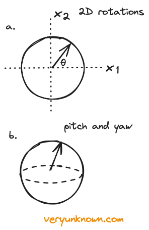
Fig 1. a) rotation in 2D
b) sphere describing pitch
and yaw, but not roll
Our starting motivation will be rather prosaic desire driven by engineering needs - what would be the mathematics to describe 3D rotations? To get going on the topic our first step will be even more basic - what would be the mathematics to describe 2D rotations? We could describe any rotation of an object with a circle as in Fig 1a, where each point of the circle represents a rotation by some angle [4]. The circle of radius one is described with equation \(x_1^2 + x_2^2 = 1\) or if we prefer using angle as parameter \(\theta\) describing angle of rotation \(x_1 = \sin\theta\), \(x_2 = \cos\theta\) then \(\sin^2 \theta + \cos^2 \theta = 1\).
Well, that was quite easy. How about 3D? In 3D to describe all rotations we need to specify three things - to borrow terminology from aeronautics we need pitch, yaw, and roll. Pitch refers to up-and-down movement (like nodding), roll to side-to-side tilting (like leaning), and yaw to left-and-right turning (like shaking one’s head). In the 2D case, we could describe rotation with one circle - making a naive guess, could we use a sphere for the 3D case? The answer is no. See Fig 1b where a point on the sphere could describe how the object has been orientated with pitch and yaw, but the roll would be missing. Now, by rough intuition, going to the sphere helped us to go from rotation like a clock, to two directions of rotation (pitch and yaw). How about going to a sphere within 4D, would points of such a sphere allow us to describe rotations fully in 3D - pitch, yaw, and roll? The answer is yes, but to see that we need to build up a bit more solid ground, so we shall do some simple algebra and we will extend from the 2D case.
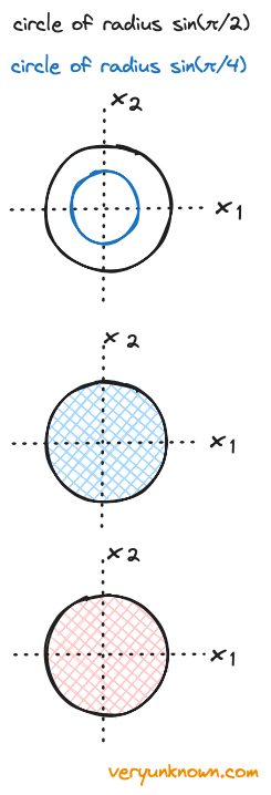
Fig 2. Circles of different radius,
eventually forming two discs
To refresh, in the 2D case, we described orientation by \(x_1^2 + x_2^2 = 1\) or if using angle as parameter \(\theta_1\) then \(\sin^2 \theta_1 + \cos^2 \theta_1 = 1\), where \(\theta_1\) is in range from 0° to 360°. Before moving forwards let us do a bit of preparation - we multiply both sides by \(\sin^2\theta_2\), where \(\theta_2\) is in range from 0° to 180°, getting \((\sin^2\theta_1 + \cos^2\theta_1)\sin^2\theta_2 = \sin^2\theta_2\). One can see that a set of \((x_1, x_2)\) points form a circle where \(x_1 = \sin\theta_1\sin\theta_2, x_2 = \cos\theta_1\sin\theta_2\), but with radius \(\sin\theta_2\) in Fig 2. If we color for all possible values by tracing out all points \(\theta_1\) and \(\theta_2\), we get two filled-in discs glued together along the edges. One disc comes from \(\theta_2\) ranges of 0° to 90°, and the second one from 90° to 180° range.
Returning back to a sphere in 3D, it would be described by \(x_1^2 + x_2^2 + x_3^2 = 1\). Note, that we could introduce new parameter \(x_3 = \cos\theta_2\) [5] and get \(x_1^2 + x_2^2 + \cos^2\theta_2 = 1\), and as \(\sin^2\theta_2 + \cos^2\theta_2 = 1\), require that \(x_1^2 + x_2^2 = \sin^2\theta_2\), and recalling prior paragraph and putting it all together \((\sin^2\theta_1 + \cos^2\theta_1)\sin^2\theta_2 + \cos^2\theta_2 = 1\).
This has been a bit lengthy route to find that we could parameterize sphere by \(x_1 = \sin\theta_1\sin\theta_2\), \(x_2 = \cos\theta_1\sin\theta_2\), \(x_3 = \cos\theta_2\), which in itself is not important for our discussion. What is important is to note that we could describe all points of a sphere by points \((x_1, x_2)\) forming the term \((\sin^2\theta_1 + \cos^2\theta_1)\sin^2\theta_2\), and which as noted before can be seen to form two discs. Another way to see that for the 3D case is that two discs represent mappings of all points of a sphere - where the top half the of sphere is one disc, the bottom half of the sphere the other, and the equator is the boundary gluing the discs in Fig 3.
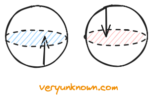
Fig 3. Sphere as two discs
We have laid the groundwork for the 4D sphere. To describe fully 3D rotations, we need three angles. So we extend the prior discussion directly with a new angle \(\theta_3\) again in range from 0° to 180°, thus allowing all values \(x_4 = \cos\theta_3\) which allows for 4D sphere of radius 1. Then we follow exactly the discussion as we did for the sphere arriving at \(((\sin^2\theta_1 + \cos^2\theta_1)\sin^2\theta_2 + \cos^2\theta_2)\sin^2\theta_3 + \cos^2\theta_3 = 1\). If we follow the same reasoning as before of mapping the points \(((\sin^2\theta_1 + \cos^2\theta_1)\sin^2\theta_2 + \cos^2\theta_2)\sin^2\theta_3\), instead of getting two discs for the 3D case, we get two spheres with filled volumes and glued surfaces as in Fig 4. In this case, we cannot visualize in picture mapping as we did for the 3D sphere in Fig 3, as we cannot really draw 4D spheres, but the same intuition applies.
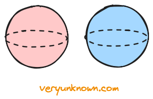
Fig 4. A sphere in 4D as two
spherical volumes
The mathematicl misfit - double cover
Having a go representing all 3D rotations as a 4D sphere is very nice. Everything looks uniform and smooth on the surface of the 4D sphere as what can be more symmetric than a sphere. As we cannot imagine a sphere in 4D, we have visualized it as two 3D balls (a ball is a filled-up sphere). As in the 2D case in Fig 1a, each point within these balls represents some sort of rotation, the question being - what rotation exactly? One idea would be to try extending Fig 1b - a layer in the volume like an onion shell gives a sphere, where a point on the onion layer would specify yaw and pitch, but in addition to Fig 1b, we could also define roll by the radius of the shell. This is a pretty intuitive starting bet, but there is a problem. A single point, the center of the ball would describe all rotations with no roll but any yaw and pitch, and we want that one point represents one unique rotation. So this representation doesn’t quite work, but let us modify it by keeping the idea that distance from origin describes the “amount of rotation” at least in some direction. Which direction? We would define the rotation to be in the direction perpendicular to an arrow. That is in Fig 5a the direction of rotation is the direction of rotation of the white disk, while the length of the arrow represents the amount of rotation.
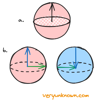
Fig 5. a) Representing rotation
as arrow b) 360° rotations
This representation is better - there are three perpendicular directions from the origin outwards, where each direction in effect describes the amount of pitch, yaw, and roll rotations, with diagonal direction describing some intermingled direction of rotation. We are pretty close to being done with describing any 3D rotation, but there is one outstanding issue with this representation. How far can the arrow extend? If we keep extending, it means we keep rotating, and then from Fig 5b we see that rotation in any two different directions (e.g. let us take pitch and yaw, green and blue respectively) eventually crosses into the second ball, and arrives at the center of the second ball. Now for this to be sensible, it is clear that for an object to be in an identical state after rotating in any direction, it must have been rotated by 360°. It is worth noting that the arrow of half the length would rotate by 180° which is the edge of one of the balls. If as an example we consider the blue rotation within the red sphere then the north pole describes rotation by 180°, while the south pole describes rotation in the opposite direction by 180°. In total, we can describe 360° rotation in any direction. So a single ball suffices to describe all 3D rotations [6].
We have finally arrived at our final description of 3D rotations - by points within a solid ball. This is all very nice but with one problem. If we come back to the 4D sphere a single ball are points of half of the sphere within 4D. What are we to do with the other half, aka the other solid ball? This is slightly a nuisance, we almost got a perfect description for our 3D rotation problem. Going back to \(x_1^2 + x_2^2 + x_3^2 + x_4^2 = 1\), we will say that list of points \((x_1, x_2, x_3, x_4)\) and \((-x_1, -x_2, -x_3, -x_4)\) describe the same rotation (where positive numbers is one of the balls, and the negatives are the other ball). This is known as “double cover”. To summarise:
3D rotations can be described as points on a half sphere within 4D space
The spooky fit - spinors
![Fig 6. An example of something spinorial [7]](/post/spinors/spinors-belt-trick.gif)
Fig 6. An example of something
spinorial [7]
With this, we can satisfy our engineering and physics needs. The pair of list of numbers \((x_1, x_2, x_3, x_4)\), and \((-x_1, -x_2, -x_3, -x_4)\) with \(x_1^2 + x_2^2 + x_3^2 + x_4^2 = 1\) will describe a 3D rotation, and we can sweep the observation of “double cover” under the rug as mathematical trivia. These are the steps of Jules Verne. But here is the absolute surprise, which is not a mathematical but physical one - there are actually objects in nature whose rotations are described solely by points \((x_1, x_2, x_3, x_4)\)! They are called “spinorial” objects, and when they are rotated by 360° they “transform to their negative”. In other words, each point of the two solid spheres describe a rotation of the spinor. What it means in the physical world is that we can take a spinorial object, and rotate it by 360°, but it does not come back to what it was - one needs to rotate it 360° again or in other words 720° in total to return to original state! This is… kind of crazy.
What examples of “spinorial objects” are there in practice? As an initial example, we can look at Fig 6. It is quite mesmerizing, but there is no trick in the picture. After 720° rotation the cube with the attached belts returns back to the initial arrangement. It is the twist in the belts that one needs to keep accounting for after 360° rotation and which makes the object “spinorial”. A much more important example is that it turns out that every particle in the physical world falls into one of the two buckets - spinorial or not. Furthermore, all particles that we think of as “stuff” are spinorial e.g. electrons, protons, neutrons, etc, while particles we think of as “forces” are not e.g. photons. Behavior under rotation is a distinguishing property of “stuff” particles and “force” particles. In short:
Rotation of spinorial objects can be described by the whole sphere within 4D space. All “stuff” particles are spinorial, while “force” particles are not.
We have made a journey from trying to describe 3D rotations, to by the end noticing that there is something that could be considered a mathematical misfit from the practical point of view or just an abstract curiosity in our description. However, it turns out that actually curiously the mathematics applies to the natural world, and in a very fundamental way. There was more in the mathematics than we originally bargained for, but it turned out to be a perfect fit. Mathematics pointed us further than initially one would have expected. As Wigner noted at the start, it is a “wonderful gift”.
[1] “Unreasonable Effectiveness of Mathematics in Physics” E. Wigner
[2] The approach was done with hindsight. The original motivation for special relativity came from electromagnetism, and in particular the mathematical implications of Maxwell’s Equations. Einstein’s famous 1905 special relativity paper was titled “Zur Elektrodynamik bewegter Körper” or in English “On the Electrodynamics of Moving Bodies”
[3] For the buffs - we will talk about SU(2) being a double cover of SO(3) by elementary means, with the remarkable fact that double cover is not just a mathematical game of Trivial Pursuits, but describes the actual natural world
[4] More commonly we think about an object as something that can be rotated, but we are taking a different view here where a shape represents all possible rotations where each point on it defines a specific rotation
[5] Where as noted previously we constrained \(\theta_2\) to be in 0° to 180° range forming a one to one map with all possible values of x which can be in range from -1 to 1
[6] A natural question to ask next would be, can our representation handle combining two rotations? The answer is yes, but we shall avoid digressing
[7] Animation of Dirac belt trick by J. Hise